Download
1 / 52
520 likes | 582 Views
What is Missing In Climate Change Assessments and Why: Unresolved Issues With the Assessment of Multi-Decadal Global Land-Surface Temperature Trends.

E N D
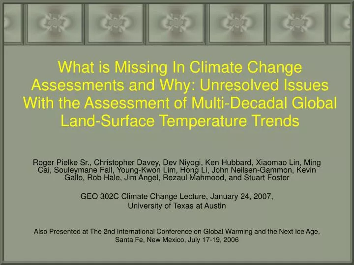
What is Missing In Climate Change Assessments and Why: Unresolved Issues With the Assessment of Multi-Decadal Global Land-Surface Temperature Trends Roger Pielke Sr., Christopher Davey, Dev Niyogi, Ken Hubbard, Xiaomao Lin, Ming Cai, Souleymane Fall, Young-Kwon Lim, Hong Li, John Neilsen-Gammon, Kevin Gallo, Rob Hale, Jim Angel, Rezaul Mahmood, and Stuart Foster GEO 302C Climate Change Lecture, January 24, 2007, University of Texas at Austin Also Presented at The 2nd International Conference on Global Warming and the Next Ice Age, Santa Fe, New Mexico, July 17-19, 2006
Davey and Pielke (2005) presented photographic documentation of poor observation sites within the U.S. Historical Climate Reference (USHCN) with respect to monitoring long term surface air temperature trends. Peterson (2006) compared the adjusted climate records of many of these stations and concluded that “…homogeneity adjusted time series from stations with poor current siting represent the temperature variability and change in the region as a whole quite well as they are almost identical to the time series from stations with excellent siting.”
One of the objectives of the USHCN as stated in Easterling et al (1996), “...was to detect temporal changes in regional rather than local climate. Therefore, only stations not influenced to any substantial degree by artificial changes in their local environments were included in the network.” Peterson’s claim relaxes this requirement with the assertion that poor station data can be corrected, so as to represent regional changes. There remain significant issues, however, with the methodology applied and the conclusion reached in the Peterson article.
dH/dt = f – T’/λ H= the heat content of the land-ocean-atmosphere system f is the radiative forcing at the tropopause T′ is the change in surface temperature λ is the climate feedback parameter T′ > 0 is GLOBAL WARMING
What is the Height of the Global Average Surface Temperature?2 m? The Actual Surface?
Influence of Height of Surface Temperature Observation on Trends - The Identification of a Warm Bias in Nighttime Minimum Temperatures
Figure 1. Δθ(z) (SBL strength) profile in different wind conditions for cases of -10 W m-2 constant cooling rate over night. From: Pielke Sr., R.A., and T. Matsui, 2005: Should light wind and windy nights have the same temperature trends at individual levels even if the boundary layer averaged heat content change is the same? Geophys. Res. Letts., 32, No. 21, L21813, 10.1029/2005GL024407.http://blue.atmos.colostate.edu/publications/pdf/R-302.pdf
Figure 2. Lapse rate of potential temperature profile for the lowest 0~10 m for different wind conditions and five different values of the flux divergence. From: Pielke Sr., R.A., and T. Matsui, 2005: Should light wind and windy nights have the same temperature trends at individual levels even if the boundary layer averaged heat content change is the same? Geophys. Res. Letts., 32, No. 21, L21813, 10.1029/2005GL024407.http://blue.atmos.colostate.edu/publications/pdf/R-302.pdf
“Most of the recent warming has been in winter over the high mid-latitudes of the Northern Hemisphere continents, between 40 and 70° N (Nicholls et al., 1996). There has also been a general trend toward reduced diurnal temperature range, mostly because nights have warmed more than days. Since 1950, minimum temperatures on land have increased about twice as fast as maximum temperatures (Easterling et al., 1997). This may be attributable in part to increasing cloudiness, which reduces daytime warming by reflection of sunlight and retards the nighttime loss of heat (Karl et al., 1997)…….”
Figure 3. Potential temperature increase at different levels from the experiment with −49 W m-2 cooling to the experiment with −50 W m-2 cooling. From: Pielke Sr., R.A., and T. Matsui, 2005: Should light wind and windy nights have the same temperature trends at individual levels even if the boundary layer averaged heat content change is the same? Geophys. Res. Letts., 32, No. 21, L21813, 10.1029/2005GL024407.http://blue.atmos.colostate.edu/publications/pdf/R-302.pdf
From: Pielke Sr., R.A., and T. Matsui, 2005: Should light wind and windy nights have the same temperature trends at individual levels even if the boundary layer averaged heat content change is the same? Geophys. Res. Letts., 32, No. 21, L21813, 10.1029/2005GL024407.http://blue.atmos.colostate.edu/publications/pdf/R-302.pdf
Further Examples of the Photographic Documentation of Poor HCN Sitings
Peterson (2006) concluded that any biases associated with poor siting can be adjusted for Peterson, T.C., 2006. Examination of potential biases in air temperature caused by poor station locations. Bull. Amer. Meteor. Soc., accepted. Pielke Sr., R.A, C. Davey, J. Angel, O. Bliss, M. Cai, N. Doesken, S. Fall, K. Gallo, R. Hale, K.G. Hubbard, H. Li, X. Lin, J. Nielsen-Gammon, D. Niyogi, and S. Raman2006, "Documentation of bias associated with surface temperature measurement sites."Bull. Amer. Meteor. Soc., submitted
Shows a large parking lot about 50 or so feet away from the temperature sensor. Station is located within 20-30 feet from the antenna. These photos are courtesy of Professor Rezaul Mahmood, Western Kentucky University, Bowling Green, KY
Shows the rain gauges and the temperature sensor's shelter. Note that the Shelter and the sensor is located over a gravel covered surface. Trees are about 20 feet from the sensor and we have no record of the growth of this tree or its maintenance (e.g., trimming).
Published other examples are in • Davey, C.A., and R.A. Pielke Sr., 2005: Microclimate exposures of surface-based weather stations - implications for the assessment of long-term temperature trends. Bull. Amer. Meteor. Soc., 86, 497–504. • Christy, J.R., 2002: When was the hottest summer? A State Climatologist struggles for an answer. Bull. Amer. Meteor. Soc. 83, 723-734. • Christy, J.R., W.B. Norris, K. Redmond and K.P. Gallo, 2006: Methodology and results of calculating Central California surface temperature trends: J. Climate, 19, 548-563. • Mahmood, R. , S.A. Foster, and David Logan, 2006: The GeoProfile metadata, exposure of instruments, and measurement bias in climatic record revisited. International Journal of Climatology, 26, 1091-1124
Influence of Trends in Surface Air Water Vapor Content on Temperature Trends
The heat content of surface air is given by H = CpT + L q This equation can be rewritten in terms of change of δT as a function of δq as δT = (L / Cp) δq
A daily composite of air temperature (red line) and effective temperature (blue line). The composite is created by averaging hourly data during the five days with highest air temperature in each of the three years considered in this section – fifteen days total. This shows the pattern of heating and cooling on the station’s extreme hottest days. Note how the effective temperature peaks approximately four hours before the air temperature peaks. Typically, the hottest days are characterized by exceptionally low relative humidity in the late afternoon, which explains the premature drop in effective temperature. From Pielke, R.A. Sr., K. Wolter, O. Bliss, N. Doesken, and B. McNoldy, 2006: The July 2005 Denver heat wave: How unusual was it? National Weather Digest, accepted for publication. http://blue.atmos.colostate.edu/publications/pdf/R-313.pdf
Annually-averaged q trends for 1982-1997, as a function of the land-cover classes listed in Table 1. All individual trends are considered and are weighted equally. From Davey, C.A., R.A. Pielke Sr., and K.P. Gallo, 2006: Differences between near-surface equivalent temperature and temperature trends for the eastern United States - Equivalent temperature as an alternative measure of heat content. Global and Planetary Change, accepted.http://blue.atmos.colostate.edu/publications/pdf/R-268.pdf
If a surface measuring site (e.g., an HCN site) undergoes a local reduction in tree cover such that as a result q decreases, then even if the value of H were unchanged, there will be an increase in surface air temperature.
A 1°C change in dewpoint temperature from 23°C to 24°C at 1000 mbar (which changes q from 18 to 19 g/ kg), for example, produces a 2.5°C change in ΔT. In other words, with the temperatures used here, the air temperature would have to increase by 2.5°C to produce the same change in H as a 1°C increase in dewpoint temperature
Degree of Independence of Land-Surface Global-Surface Temperature Analyses Tropical regions have sparse coverage of surface temperature data. Until further information can be obtained in these regions, the robustness of warming estimates in this region should be questioned. Thus the CCSP (2006) finding that the “the majority of observational data sets show more warming at the surface than in the troposphere,” while “ all model simulations show more warming in the troposphere than at the surface” may be a result of the inadequate sampling of the tropical land areas.
Five latitudinal bands designated corresponding to the polar (>50N,>50S), temperate (20N-50N,20S-50S, and tropical (20N-20S) regions of the world. From Davey and Pielke, 2006: Comparing station density and reported temperature trends for land surface sites, 1979-2004. Climatic Change, submitted.
Percent of Land Grid Points that Have Different Numbers of Surface Temperature Observing SitesAbout 70% of the grid points have one or less observing sites!
Relationship Between In-Situ Surface Temperature Observations and the Diagnosis of Surface Temperature Trends from North American Regional Reanalysis
Monthly mean temperature anomalies (curves; unit: C) at Trinidad and their linear trends (lines).
Same as previous figure except for the station Cheyenne Wells.
The same as the previous figure except for the station Las Animas.
The same as the previous figure except for the station Eads.
The same as the previous figure except for the station Lamar.
Standard deviation of the monthly mean temperature anomalies
Linear regression trends of the monthly mean temperature anomalies (Unit: C/10years)
Influence of Land Use/Land Cover Change on Surface Temperature Trends Hale, R.C., K.P. Gallo, T.W. Owen, and T.R. Loveland, 2006: Land Use/Land Cover Change Effects on Temperature Trends at U.S. Climate Normals Stations. Geophys. Res. Lett., 33, L11703, doi:10.1029/2006GL026358, 2006 “Results indicate relatively few significant temperature trends before periods of greatest LULC change, and these are generally evenly divided between warming and cooling trends. In contrast, after the period of greatest LULC change was observed, 95% of the stations that exhibited significant trends (minimum, maximum, or mean temperature) displayed warming trends.”
Vegetation Greenness Impacts on Maximum and Minimum Temperatures in Northeast Colorado “At most sites, there is a seasonal dependence in the explained variance of the minimum and maximum temperatures because of the seasonal cycle of plant growth and senescence. Between individual sites, the highest increase in explained variance occurred at the site with the least amount of anthropogenic influence. This work suggests the vegetation state needs to be included as a factor in surface temperature forecasting, numerical modeling, and climate change assessments.” See Hanamean, J.R. Jr., R.A. Pielke Sr., C.L. Castro, D.S. Ojima, B.C. Reed, and Z. Gao, 2003: Vegetation impacts on maximum and minimum temperatures in northeast Colorado. Meteorological Applications, 10, 203-215. http://blue.atmos.colostate.edu/publications/pdf/R-254.pdf
5 km radius circle of 30 m resolution land-use data for Fort Collins. The color scales represent: purple - low and high intensity residential/commercial/industrial/ transportation; orange - grasslands/herbaceous; and dark red – herbaceous planted/cultivated. Other land-use covers an area of less than 1%.
5 km radius circle of 30 m resolution land-use data for Fort Morgan. The color scales represent: purple - low and high intensity residential/commercial/industrial/ transportation; orange - grasslands/herbaceous; and dark red – herbaceous planted/cultivated. Other land-use covers an area of less than 1%.
5 km radius circle of 30 m resolution land-use data for Wray. The color scales represent: purple - low and high intensity residential/commercial/industrial/ transportation; orange - grasslands/herbaceous; and dark red – herbaceous planted/cultivated. Other land-use covers an area of less than 1%.
Averaged r2 differences. Time blocks for the years 1989-1998. Maximum temperatures. Shows the r2 difference between the 850-700 mb layer mean temperature maxima correlated to the surface temperature maxima subtracted from the same layer mean temperature extrema including vegetation impacts via NDVI values correlated to the surface temperature extrema. Values are significant to 95 percent confidence level.
Averaged r2 differences. Time blocks for the years 1989-1998. Minimum temperatures. Shows the r2 difference between the 850-700 mb layer mean temperature minimum correlated to the surface temperature minimum subtracted from the same layer mean temperature extrema including vegetation impacts via NDVI values correlated to the surface temperature extrema. Values are significant to 95 percent confidence level.
Other Issues To Be Elaborated on in the JGR Paper • Undocumented station changes • Uncertainties in adjustments • Impact of adjustments on estimated climate trends
The Reason for the Lack of Recognition of the Problems with the Surface Temperature Trend Data is Due to the Conflict of Interest in Preparing such Climate Assessments
Preface Exec Summ Chap 1 Chap 2 Chap 3 Chap 4 Chap 5 Chap 6 Append A CCSP REPORTPreface. Report Motivation and Guidance for Using this Synthesis/Assessment Report by Karl, T.R., C. D. Miller, and W. L. Murray, editorExecutive Summary by Wigley, T.M.L., V. Ramaswamy, J.R. Christy, J.R. Lanzante, C.A. Mears, B.D. Santer, C.K. FollandChapter 1 . Why do temperatures vary vertically (from the surface to the stratosphere) and what do we understand about why they might vary and change over time? by Ramaswamy, V., J.W. Hurrell, G.A. MeehlChapter 2. What kinds of atmospheric temperature variations can the current observing systems measure and what are their strengths and limitations, both spatially and temporally? by Christy, J.R., D.J. Seidel, S.C. SherwoodChapter 3. What do observations indicate about the changes of temperature in the atmosphere and at the surface since the advent of measuring temperatures vertically? by Lanzante, J.R., T.C. Peterson, F.J. Wentz, K.Y. VinnikovChapter 4. What is our understanding of the contribution made by observational or methodological uncertainties to the previously reported vertical differences in temperature trends? by Mears, C.A., C.E. Forest, R.W. Spencer, R.S. Vose, R.W. ReynoldsChapter 5. How well can the observed vertical temperature changes be reconciled with our understanding of the causes of these temperature changes? by Santer, B.D., J.E. Penner, P.W. ThorneChapter 6. What measures can be taken to improve our understanding of observed changes? by Folland, C.K., D. Parker, R.W. Reynolds, S.C. Sherwood, P.W. ThorneAppendix A. Statistical Issues Regarding Trends. by Wigley, T.M.L. Santer, B.D., T.M.L. Wigley, C. Mears, F.J. Wentz, S.A. Klein, D.J. Seidel, K.E. Taylor, P.W. Thorne, M.F. Wehner, P.J. Gleckler, J.S. Boyle, W.D. Collins, K.W. Dixon, C. Doutriaux, M. Free, Q. Fu, J.E. Hansen, G.S. Jones, R. Ruedy, T.R. Karl, J.R. Lanzante, G.A. Meehl, V. Ramaswamy, G. Russel, and G.A. Schmidt, 2005: Amplification of surface temperature trends and variability in the tropical atmosphere. Science, 309, 1551- 1556. DOI:10.1126/science.1114867. Mears, C.A., and F.J. Wentz, 2005: The effect of diurnal correction on satellite-derived lower tropospheric temperature. Science, 1548-1551. doi:10.1126/science.1114772. Sherwood, S.C., J.R. Lanzante, and C.L. Meyer, 2005: Radiosonde daytime biases and late-20th century warming. Science, 1556-1559.doi:10.1126/science.1115640.
CONCLUSIONS • The objective of the research is to evaluate long-term surface temperature monitoring sites for use in regional and global surface temperature trend analyses. • We find a variety of significant issues on the quantitative accuracy of the reported analyses • This raises concerns on their use to evaluate a global average surface temperature trend • The use of ocean heat content changes over time is the recommended metric for the assessment of variations and trends in climate system heat content.