Download
1 / 43
430 likes | 603 Views
Theoretical Approaches to Machine Learning. Early work (eg. Gold) ignored efficiency Only considers computability “Learning in the limit” Later work considers tractable i nductive learning With high probability, approximately learn Polynomial runtime, polynomial # of examples needed

E N D
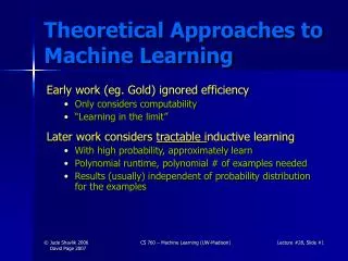
Theoretical Approaches to Machine Learning Early work (eg. Gold) ignored efficiency • Only considers computability • “Learning in the limit” Later work considers tractable inductive learning • With high probability, approximately learn • Polynomial runtime, polynomial # of examples needed • Results (usually) independent of probability distribution for the examples CS 760 – Machine Learning (UW-Madison)
Identification in the Limit DefinitionAfter some finite number of examples, learner will have learned the correct concept (though might not even know it!). Correct means agrees with target concept on labels for all data. ExampleConsider noise-free learning from the class {f | f(n) = a*n mod b} where a and b are natural numbers General Technique “Innocent Until Proven Guilty” Enumerate all possible answers Search for simplest answer consistent with training examples seen so far; sooner or later will hit solution CS 760 – Machine Learning (UW-Madison)
Some Results (Gold) • Computable languages (Turing machines) can be learned in the limit using inference by enumeration. • If data set is limited to positive examples only, then only finite languages can be learned in the limit. CS 760 – Machine Learning (UW-Madison)
Solution for {f | f(n) = a*n mod b} b n f(n) 9 17 a CS 760 – Machine Learning (UW-Madison)
The Mistake-Bound Model (Littlestone) Framework • Teacher shows input I • ML algorithm guesses output O • Teacher shows correct answer • Can we upper bound the number of errors the learner will make? CS 760 – Machine Learning (UW-Madison)
The Mistake-Bound Model Example Learn a conjunct from N predicates and their negations • Initial h = p1 ¬p1 … pn ¬pn • For each + ex, remove the remaining terms that do not match CS 760 – Machine Learning (UW-Madison)
The Mistake-Bound Model Worst case # of mistakes? 1 + N • First + ex will remove Nterms from hinitial • Each subsequent error on a + will remove at least one more term (never make a mistake on - ex’s) CS 760 – Machine Learning (UW-Madison)
Equivalence Query Model (Angluin) Framework • ML algorithm guesses concept: is target equivalent to this guess?) • Teacher either says “yes” or returns a counterexample (example labeled differently by target and guess) • Can we upper bound the number of errors the learner will make? • Time to compute next guess bounded by Poly(|data seen so far|) CS 760 – Machine Learning (UW-Madison)
Probably Approximately Correct (PAC) Learning PAC learning (Valiant ’84) Given X domain of possible examples C class of possible concepts to label X c C target concept , correctness bounds CS 760 – Machine Learning (UW-Madison)
Probably Approximately Correct (PAC) Learning • For any target c in C and any distribution D on X • Given at least N = poly(|c|,1/e,1/d) examples drawn randomly, independently from X • Do with probability 1 - , return an h in Cwhose accuracy is at least 1 - • In other words Prob[error(h, c) > ] < • In time polynomial in |data| c Shaded regions are where errors occur: h CS 760 – Machine Learning (UW-Madison)
Relationships Among Models of Tractable Learning • Poly mistake-bounded with poly update time = EQ-learning • EQ-learning implies PAC-learning • Simulate teacher by poly-sized random sample; if all labeled correctly, say “yes”; otherwise, return incorrect example • On each query, increase sample size based on Bonferoni correction CS 760 – Machine Learning (UW-Madison)
To Prove Concept Class is PAC-learnable • Show it’s EQ-learnable, OR • Show the following: • There exists an efficient algorithm for the consistency problem (find a hypothesis consistent with a data set in time poly in the size of the data set) • Poly-sized sample is sufficient to give us our accuracy guarantees CS 760 – Machine Learning (UW-Madison)
Useful Trick:A Maclaurin series: for -1 < x <= 1:We only care about -1<x<0. Rewriting -x as ε, we can derive that for 0<ε<1: ln(1-ε) <= -ε.Because ε is positive, we can put both sides of this last inequality into an exponent to obtain: 1 - ε <= e-ε CS 760 – Machine Learning (UW-Madison)
Assume EQ Query Bound (or Mistake Bound) M • On each equivalence query, draw: 1/εln(M/δ) examples • What is the probability that on any of the at most M rounds, we accept a “bad” hypothesis? • At most M (1-ε)1/εln(M/δ) <= M e-ln(M/δ) (using the useful trick) = δ CS 760 – Machine Learning (UW-Madison)
If Algorithm Doesn’t Know M in Advance (recall |c|): • On ith equivalence query, draw: 1/ε (ln(1/δ) + iln(2)) examples • What is the probability that we accept a “bad” hypothesis at one query? • (1-ε)1/ε (ln(1/δ) + iln(2)) <= e- (ln(1/δ) + iln(2)) (using the useful trick) = δ/2i • So probability we ever accept a “bad” hypothesis is at most δ. CS 760 – Machine Learning (UW-Madison)
Using First Method: kDNF • Write down disjunction of all conjunctions of at most k literals (features or negated features) • Any counterexample will be actual negative • Repeat until correct: Given a counterexample, delete disjuncts that cover it (are consistent with it) CS 760 – Machine Learning (UW-Madison)
Using Second Method • If hypothesis space is finite, can show a poly sample is sufficient • If hypothesis space is parameterized by n, and grows only exponentially in n, can show a poly sample is sufficient CS 760 – Machine Learning (UW-Madison)
How Many Examples Needed to be PAC? • Consider finite hypothesis spaces • Let Hbad {h1, …, hz} • The set of hypotheses whose (“testset”) error is > • Goal Eliminate all items in Hbadvia (noise-free) training examples CS 760 – Machine Learning (UW-Madison)
How Many Examples Needed to be PAC? How can an h look bad, even though it is correct on all the training examples? • If we never see any examples in the shaded regions • We’ll compute an N s.t. the odds of this are sufficiently low (recall, N = number of examples) c h CS 760 – Machine Learning (UW-Madison)
Hbad • Consider H1 Hbad and ex N • What is the probability that H1 is consistent with ex? Prob[consistentA(ex,H1)] ≤ 1 - (since H1 is bad its error rate is at least ) CS 760 – Machine Learning (UW-Madison)
Hbad (cont.) What is the probability that H1 is consistent with allN examples? Prob[consistentB(N,H1)] ≤ (1 - )|N| (by iid assumption) CS 760 – Machine Learning (UW-Madison)
Hbad (cont.) What is the probability that some member of Hbad is consistent with the examples in N ? Prob[consistentC(N, Hbad)] Prob[consistentB(N, H1) … consistentB(N, Hz)] ≤ |Hbad| x (1-)|N| //P(AB) P(A) + P(B) - P(AB) ≤ |H| x (1- )|N| // Hbad H Ignore this in upper bound calc CS 760 – Machine Learning (UW-Madison)
Solving for |N| We have Prob[consistentC(N,Hbad)] ≤ |H| x (1-)|N| < Recall that we want the prob of a bad concept surviving to be less than , our bound on learning a poor concept Assume that if many consistent hypotheses survive, we get unlucky and choose a bad one (we’re doing a worst-case analysis) CS 760 – Machine Learning (UW-Madison)
Solving for |N|(number of examples needed to be confident of getting a good model) Solving |N| > [ln(1/)+ln(|H|)] / -ln(1-) Since ≤ -ln(1-) over [0,1) we get |N| > [ln(1/)+ln(|H|)] / (Aside: notice that this calculation assumed we could always find a hypothesis that fits the training data) Notice we made NO assumptions about the prob dist of the data (other than it does not change) CS 760 – Machine Learning (UW-Madison)
Example: Number of Instances Needed Assume F = 100 binary features H = all (pure) conjuncts [3F possibilities (i, use fi, use ¬fi, or ignore fi) so lg|H| = F * lg 3 ≈ F] = 0.01 = 0.01 N = [ln(1/)+ln(|H|)] / = 100 * [ln(100) + 100] ≈ 104 But how many real-world concepts are pure conjuncts with noise-free training data? CS 760 – Machine Learning (UW-Madison)
Two Senses of Complexity Sample complexity(number of examples needed) vs. Time complexity(time needed to find h H that is consistent with the training examples) CS 760 – Machine Learning (UW-Madison)
Complexity (cont.) • Some concepts require a polynomial number of examples but an exponential amount of time (in the worst case) • Eg, training neural networks is NP-hard (recall BP is a “greedy” algorithm that finds a local min) CS 760 – Machine Learning (UW-Madison)
Dealing with Infinite Hypothesis Spaces • Can use the Vapnik-Chervonenkis (‘71) dimension (VC-dim) • Provides a measure of the capacity of a hypothesis space VC-dim given a hypothesis space H, the VC-dim is the size of the largest set of examples that can be completely fit by H, no matter how the examples are labeled CS 760 – Machine Learning (UW-Madison)
VC-dim Impact • If the number of examples << VC-dim, then memorizing training is trivial and generalization likely to be poor • If the number of examples >> VC-dim, then the algorithm must generalize to do well on the training set and will likely do well in the future CS 760 – Machine Learning (UW-Madison)
Samples of VC-dim Finite H VC-Dim ≤ log2|H| (if d examples, 2d different labelings possible, and must have 2d ≤ |H| if all functions are to be in H) CS 760 – Machine Learning (UW-Madison)
An Infinite Hypothesis Space with a Finite VC Dim H is set of lines in 2D Can cover 1 ex no matter how labeled 1 CS 760 – Machine Learning (UW-Madison)
Example 2 (cont.) Can cover 2 ex’s no matter how labeled 2 1 CS 760 – Machine Learning (UW-Madison)
Example 2 (cont.) Can cover 3 ex’s no matter how labeled 1 2 3 CS 760 – Machine Learning (UW-Madison)
Example 2 (cont.) Cannot cover/separate if 1 and 4 are +, But 2 and 3 are – (our old friend, ex-or) • Notice |H| = ∞ but VC-dim = 3 • For N-dimensions and N-1 dim hyperplanes,VC-dim = N + 1 2 1 4 3 CS 760 – Machine Learning (UW-Madison)
More on “Shattering” What about collinear points? If some set of d examples that H can fully fit labellings of these d examples then VC(H) ≥ d CS 760 – Machine Learning (UW-Madison)
Some VC-Dim Theorems TheoremH is PAC-learnable iff its VC-dim is finite TheoremSufficient to be PAC to have # of examples > 1/ max[4ln(2/), 8ln(13/)VC-dim(H)] TheoremAny PAC algorithm needs at least (1/[ln(1/) + VC-dim(H)]) examples [No need to memorize these for the exam] CS 760 – Machine Learning (UW-Madison)
To Show a Concept is NOT PAC-learnable • Show the consistency problem is NP-hard (hardness assumes P ≠ NP), OR • Show the VC-dimension grows at a rate not bounded by any polynomial CS 760 – Machine Learning (UW-Madison)
Be Careful • It can be the case that consistency is hard for a concept class, but not for a larger class • Consistency NP-hard for k-term DNF • Consistency easy for DNF (PAC still open ques.) • More robust negative results are for PAC-prediction • Hypothesis space not constrained to equal concept class • Hardness results based on cryptographic assumptions, such as assuming efficient factoring is impossible CS 760 – Machine Learning (UW-Madison)
Some Variations in Definitions • Original definition of PAC-learning required: • Run-time to be polynomial • Hypothesis to be within concept class (otherwise, called PAC-prediction) • Now this version is often called polynomial-time, proper PAC-learning • Membership queries: can ask for labels of specific examples CS 760 – Machine Learning (UW-Madison)
Some Results… • Can PAC-learn k-DNF (exponential in k, but k is now a constant) • Can NOTproper PAC-learn k-term DNF, but can PAC-learn it by k-CNF • Can NOT PAC-learn Boolean Formulae unless can crack RSA (can factor fast) • Can PAC-learn decision-trees with the addition of membership queries • Unknown whether can PAC-learn DNF or DTs (“holy grail” questions of COLT) CS 760 – Machine Learning (UW-Madison)
Some Other COLT Topics COLT + clustering + k-NN+ RL+ EBL (ch. 11 of Mitchell)+ SVMs+ ILP+ ANNs, etc. • Average case analysis (vs. worst case) • Learnability of natural languages (language innate?) • Learnability in parallel CS 760 – Machine Learning (UW-Madison)
Summary of COLT Strengths • Formalizes learning task • Allows for imperfections (e.g. and in PAC) • Work on boosting (later) is excellent case of ML theory influencing ML practice • Shows what concepts are intrinsically hard to learn (e.g. k-term DNF) CS 760 – Machine Learning (UW-Madison)
Summary of COLT Weaknesses • Most analyses are worst case • Use of “prior knowledge” not captured very well yet CS 760 – Machine Learning (UW-Madison)