Download
1 / 62
620 likes | 630 Views
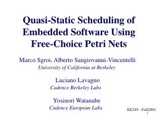
Quasi-static Scheduling for Reactive Systems. Jordi Cortadella , Universitat Politècnica de Catalunya, Spain Alex Kondratyev , Cadence Berkeley Labs, USA Luciano Lavagno , Politecnico di Torino, Italy Claudio Passerone , Politecnico di Torino, Italy

E N D
Quasi-static Scheduling for Reactive Systems Jordi Cortadella, Universitat Politècnica de Catalunya, Spain Alex Kondratyev, Cadence Berkeley Labs, USA Luciano Lavagno, Politecnico di Torino, Italy Claudio Passerone, Politecnico di Torino, Italy Yosinori Watanabe, Cadence Berkeley Labs, USA Joint work with: Robert Clarisó, Alex Kondratyev, Luciano Lavagno, Claudio Passerone and Yosinori Watanabe (UPC, Cadence Berkeley Labs, Politecnico di Torino)
Outline • The problem • Synthesis of concurrent specifications • Previous work: Dataflow networks • Static scheduling of SDF networks • Quasi-Static Scheduling of process networks • Petri net representation of process networks • Scheduling and code generation • Open problems
Embedded Software Synthesis • Specification: concurrent functional netlist (Kahn processes, dataflow actors, SDL processes, …) • Software implementation: (smaller) set of concurrent software tasks • Two sub-problems: • Generate code for each task • Schedule tasks dynamically • Goals: • minimize real-time scheduling overhead • maximize effectiveness of compilation
Temperature TSENSOR HSENSOR Humidity TEMP FILTER HUMIDITY FILTER ENVIRONMENTAL CONTROLLER TDATA HDATA CONTROLLER AC-on DRYER-on ALARM-on AC Dehumidifier Alarm Environmental controller
Environmental controller TEMP-FILTER float sample, last; last = 0; forever { sample = READ(TSENSOR); if (|sample - last| > DIF) { last = sample; WRITE(TDATA, sample); } } TSENSOR HSENSOR TEMP FILTER HUMIDITY FILTER TDATA HDATA CONTROLLER AC-on DRYER-on ALARM-on
Environmental controller TEMP-FILTER float sample, last; last = 0; forever { sample = READ(TSENSOR); if (|sample - last| > DIF) { last = sample; WRITE(TDATA, sample); } } TSENSOR HSENSOR TEMP FILTER HUMIDITY FILTER TDATA HDATA HUMIDITY-FILTER float h, max; forever { h = READ(HSENSOR); if (h > MAX) WRITE(HDATA, h); } CONTROLLER AC-on DRYER-on ALARM-on
Environmental controller CONTROLLER float tdata, hdata; forever { select(TDATA,HDATA) { case TDATA: tdata = READ(TDATA); if (tdata > TFIRE) WRITE(ALARM-on,10); else if (tdata > TMAX) WRITE(AC-on, tdata-TMAX); case HDATA: hdata = READ(HDATA); if (hdata > HMAX) WRITE(DRYER-on, 5); } } TSENSOR HSENSOR TEMP FILTER HUMIDITY FILTER TDATA HDATA CONTROLLER AC-on DRYER-on ALARM-on
TSENSOR HSENSOR TEMP FILTER HUMIDITY FILTER TDATA HDATA CONTROLLER AC-on DRYER-on ALARM-on Environ. Processes OS Tsensor T-FILTERwakes up Operating system T-FILTERexecutes T-FILTERsleeps Hsensor H-FILTERwakes up H-FILTERexecutes &sends datato HDATA H-FILTERsleeps CONTROLLERwakes up CONTROLLERexecutes &reads datafrom HDATA . . .
Operating system • Goal: improve performance • Reduce operating system overhead • Reduce communication overhead • How?: Do as much as possible statically • Scheduling • Compiler optimizations TSENSOR HSENSOR TEMP FILTER HUMIDITY FILTER TDATA HDATA CONTROLLER AC-on DRYER-on ALARM-on
Outline • The problem • Synthesis of concurrent specifications • Previous work: Dataflow networks • Static scheduling of SDF networks • Quasi-Static Scheduling of process networks • Petri net representation of process networks • Scheduling and code generation • Open problems
Intuitive semantics • (Often stateless) actors perform computation • Unbounded FIFOs perform communication via sequences of tokens carrying values • (matrix of) integer, float, fixed point • image of pixels, ….. • Determinacy: • unique output sequences given unique input sequences • Sufficient condition: blocking read (process cannot test input queues for emptiness)
Intuitive semantics • Example: FIR filter • single input sequence i(n) • single output sequence o(n) • o(n) = c1* i(n) + c2* i(n-1) i(-1) i c1 c2 + o
FFT 1024 1024 10 1 Examples of Dataflow actors • SDF: Static Dataflow: fixed number of input and output tokens • BDF: Boolean Dataflow control token determines number of consumed and produced tokens 1 + 1 1 T F select merge T F
Static scheduling of DF • Key property of DF networks: output sequences do not depend on firing sequence of actors • SDF networks can be statically scheduled at compile-time • execute an actor when it is known to be fireable • no overhead due to sequencing of concurrency • static buffer sizing • Different schedules yield different • code size • buffer size • pipeline utilization
A B np nc Balance equations • Number of produced tokens must equal number of consumed tokens on every edge • Repetitions (or firing) vector vS of schedule S: number of firings of each actor in S • vS(A) np= vS(B) nc must be satisfied for each edge nc np A B
Balance equations • Balance for each edge: • 3 vS(A) - vS(B) = 0 • vS(B) - vS(C) = 0 • 2 vS(A) - vS(C) = 0 • 2 vS(A) - vS(C) = 0 A 2 3 2 1 1 1 B C 1 1
3 -1 0 0 1 -1 2 0 -1 2 0 -1 A 2 3 M = 2 1 1 1 B C 1 1 Balance equations • M vS = 0 iff S is periodic • Full rank (as in this case) • no non-zero solution • no periodic schedule (too many tokens accumulate on AB or BC)
2 -1 0 0 1 -1 2 0 -1 2 0 -1 A 2 2 M = 2 1 1 1 B C 1 1 Balance equations • Non-full rank • infinite solutions exist (linear space of dimension 1) • Any multiple of q = |1 2 2|T satisfies the balance equations • ABCBC and ABBCC are minimal valid schedules • ABABBCBCCC is non-minimal valid schedule
A 2 2 2 1 1 1 B C 1 1 From repetition vector to schedule • Repeatedly schedule fireable actors up to number of times in repetition vector q = |1 2 2|T • Can find either ABCBC or ABBCC • If deadlock before original state, no valid schedule exists (Lee ‘86)
Compilation optimization • Assumption: code stitching (chaining custom code for each actor) • More efficient than C compiler for DSP • Comparable to hand-coding in some cases • Explicit parallelism, no artificial control dependencies • Main problem: memory and processor/FU allocation depends on scheduling, and vice-versa
Code size minimization • Assumptions (based on DSP architecture): • subroutine calls expensive • fixed iteration loops are cheap (“zero-overhead loops”) • Global optimum: single appearance schedule e.g. ABCBC A (2BC), ABBCC A (2B) (2C) • may or may not exist for an SDF graph… • buffer minimization relative to single appearance schedules (Bhattacharyya ‘94, Lauwereins ‘96, Murthy ‘97)
1 A 10 C D 1 10 B 10 1 Buffer size minimization • Assumption: no buffer sharing • Example: q = | 100 100 10 1|T • Valid SAS: (100 A) (100 B) (10 C) D • requires 210 units of buffer area • Better (factored) SAS: (10 (10 A) (10 B) C) D • requires 30 units of buffer areas, but… • requires 21 loop initiations per period (instead of 3)
Scheduling more powerful DF • SDF is limited in modeling power • More general DF is too powerful • non-Static DF is Turing-complete (Buck ‘93) • bounded-memory scheduling is not always possible • Boolean Data Flow: Quasi-Static Scheduling of special “patterns” • if-then-else, repeat-until, do-while • Dynamic Data Flow: run-time scheduling • may run out of memory or deadlock at run time • Kahn Process Networks: quasi-static scheduling using Petri nets • conservative: schedulable network may be declared unschedulable
Outline • The problem • Synthesis of concurrent specifications • Compiler optimizations across processes • Previous work: Dataflow networks • Static scheduling of SDF networks • Code and data size optimization • Quasi-Static Scheduling of process networks • Petri net representation of process networks • Scheduling and code generation • Open problems
QSS Quasi-Static Scheduling • Sequentialize concurrent operations as much as possible • less communication overhead(run-time task generation) • better starting point for compilation(straight-line code from function blocks) • Must handle • data-dependent control • multi-rate communication
The problem • Given: a network of Kahn processes • Kahn process: sequential function + ports • communication: port-based, point-to-point, uni-directional, multi-rate • Find: a single task • functionally equivalent to the originalnetwork (modulo concurrency) • driven by input stimuli(no OS intervention) TSENSOR HSENSOR TEMP FILTER HUMIDITY FILTER TDATA HDATA CONTROLLER AC-on DRYER-on ALARM-on
The scheduling procedure 1. Specify a network of processes • process: C + communication operations • netlist: connection between ports 2. Translate to the computational model: Petri nets 3. Find a “schedule” on the Petri net 4. Translate the schedule to a task
TSENSOR TSENSOR TEMP FILTER last = 0 TDATA sample = READ(TSENSOR) TEMP-FILTER float sample, last; last = 0; while (1) { sample = READ(TSENSOR); if (|sample - last|> DIF) { last = sample; WRITE(TDATA, sample); } } F T last = sample; WRITE(TDATA,sample) TDATA
Petri nets for Kahn process networks Channels (point-to-point communication between processes) Input/Output ports (communication with the environment) Sequential processes (1 token per process)
Petri nets for Kahn process networks True True False False • Data-dependent choices • Conservative assumption (any outcome is possible)
Scheduling game Adversary Scheduler t1 t2 t3 Data choice + inputs The rest of transitions t4 t5 t6 t1 t2 t4 t5 t1 t3 t6
Scheduling game Adversary Scheduler t1 t2 t3 Data choice + inputs The rest of transitions t4 t5 t6 t1 t2 t4 t5 t1 t3 t6
t4 t4 t4 t1 t2 t1 t2 t1 t2… Scheduling game Adversary Scheduler t1 t2 t3 Data choice + inputs The rest of transitions t4 t5 t6
a d a p0p1 p0 p3 p1 d p2 p0p3 e b p5 p4 p2 p4p5 g f c a d p0p5p1 p0p5 p0p3p5 p2p5 Schedule generation p0 • Schedule is an RG subset: • Finite • Sequential • Live wrt to source transitions • All FCS transitions are fired in a state (FCS: always conflicting transitions) Depth first traversal with backtracking
a d a p0 p0p1 p0 p3 p1 d p2 p0p3 e b p5 p4 p2 p4p5 g f c a d p0p5 p0p5p1 p0p3p5 • Schedule is an RG subset: • Finite • Sequential • Live wrt to source transitions • All FCS transitions are fired in a state p2p5 (FCS: always conflicting transitions) Depth first traversal with backtracking Schedule generation Await states
Handling infinity PN with source transitions has infinite reachability space Irrelevance Criterion: • Impose place “bounds” by the structure of the PN. • Identify “irrelevant nodes” in the reachability tree. • If the algorithm hits an irrelevant node, backtrack. Need for termination conditions during traversal Bounds the reachability space!!!
2 4 I - max + max - 1 - the initial marking of p o k j 3 1 u v i m i 1 o n o 1 no traversal beyond v Irrelevance criterion bound of place=max of v is irrelevant node iff: max(3+4-1, 1) = 6 1. v succeds u, 2. p, M(u, p) M(v, p), 3. p, if M(u, p) < M(v, p), then M(u, p) the bound of p. v is as at least capable as u u already hits the bounds Irrelevance is more than marking, it is marking+history!!!
p1 p3 C p2 p3 p1 A p1 p3 p4 B A 2 A p5 p4 p1 p3 p4 p4 C D E p1 p2 p4 p4 p6 B 2 p4 p4 p5 p5 E D p4 p5 p6 D p6 p6 Quality of irrelevance criterion Heuristic for the general Petri nets: irrelevant For unique and/or free choice PNs irrelevance may be exact (if yes, then schedulability is decidable in this class) Open issue
Properties of the Algorithm Claim1: • If the algorithm terminates successfully, a schedule is obtained. Claim2: • If the algorithm does NOT terminate successfully, no schedule exists under given termination conditions Semi-decision procedure!!!
Single Source Schedules a d a a p0p1 p0p1 p0 p3 SSS(d) p1 d d d p0 p2,p0 p2 p2 p0p3 p0p3 p0,p0p3 SSS(a) p0 e b p5 p4 p2 p4p5 p4p5 g f c a d d d p0p5p1 p0p5 p0p5 p0,p0p3p5 p0p3p5 p0p3p5 Schedule Composition p2p5 p2,p0p5 a p0,p0 p0p1,p0 p0 Isomorphic p0,p4p5 a p0,p0p5 p0p1,p0p5 Divide and conquer
Single Source Schedules a d a p0p1 p0 p0 p3 SSS(d) p1 d d p2,p0 p2 p0,p0p3 p0p3 SSS(a) p0 e b p5 p4p5 p4 p2 d g f p4p5p3 p0p3p5 c Composition No isomorphic schedule exists a p0,p0 p0p1,p0 a p0,p4p5 p0p1,p4p5 Independence of SSS!!! d p0,p0p5 p0,p0p3p5 p2,p4p5 Divide and conquer
Checking SSS independence Marking equations Consumption of tokens SSS independence N. and S. condition: M0(p) – worst_change(p,a) – SSS_change(p,a) 0 Worst consumption of p in SSS(a) Worst consumption of p in other SSSs Complexityof checking: O( |SSS|) Composition has exponentially larger number of states!!!
Code generation Initialization I1 system Await state I1 I2 I2 • Generated code: • ISRs driven by input stimuli (I1 and I2) • Each tasks contains threads from one await state to another await state Choice I1 I2 T F F T I1 I2
Code generation I1 system I1 I2 I2 • Generated code: • ISRs driven by input stimuli (I1 and I2) • Each tasks contains threads from one await state to another await state I1 I2 T F F T I1 I2
S1 S2 S3 Code generation Init I1 system I1 I2 I2 C9 C1 C4 • Generated code: • ISRs driven by input stimuli (I1 and I2) • Each tasks contains threads from one await state to another await state C5 C2 C3 C11 F I2 I1 I1 I2 C8 C6 C10 T C7
S1 S2 S3 Code generation enum state {S1, S2, S3} S; C0 I1 I2 C9 C1 C4 C5 C2 C3 C11 F I2 I1 I1 I2 C8 C6 C10 T C7
S1 Code generation enum state {S1, S2, S3} S; Init () { C0(); S = S1; return; } C0
S1 S2 S3 Code generation enum state {S1, S2, S3} S; ISR1 () { switch(S) { case S1: C1(); C2(); S=S2; return; case S2: C3(); C2(); return; case S3: C6(); C7(); C11(); C5(); return; } } I1 C1 C5 C2 C3 C11 I1 I1 C6 C7
S1 S2 S3 Code generation enum state {S1, S2, S3} S; ISR2 () { switch(S) { case S1: C4(); C5(); S=S3; break; case S2: C10(); C11(); C5(); S=S3; return; case S3: if (C8()) { C7(); C11(); C5(); return; } else { C9(); S = S1; return; } } } I2 C9 C4 C5 C11 F I2 I2 C8 C10 T C7
S1 S2 S3 Code generation enum state {S1, S2, S3} S; Init () { C0(); S = S1; return; } ISR1 () { switch(S) { case S1: C1(); C2(); S=S2; return; case S2: C3(); C2(); return; case S3: C6(); C7(); C11(); C5(); return; } } ISR2 () { switch(S) { case S1: C4(); C5(); S=S3; break; case S2: C10(); C11(); C5(); S=S3; return; case S3: if (C8()) { C7(); C11(); C5(); return; } else { C9(); S = S1; return; } } } C0 I1 I2 C9 C1 C4 C5 C2 C3 C11 F I2 I1 I1 I2 C8 C6 C10 T C7