Download
1 / 24
250 likes | 506 Views
Image Analysis. Preprocessing Image Quantization Binary Image Analysis Thresholding via Histogram Connectivity and Labeling. Image Quantization. is the process of reducing the image data by removing some of the detail information by mapping groups of data points to a single point.

E N D
Image Analysis Preprocessing Image Quantization Binary Image Analysis Thresholding via Histogram Connectivity and Labeling
Image Quantization • is the process of reducing the image data by removing some of the detail information by mapping groups of data points to a single point. • can be done to either the pixel values themselves, I(r, c), or to the spatial coordinates, (r, c). • Operation on the pixel values is referred to as gray level reduction, while operating on the spatial coordinates called spatial reduction.
gray level reduction • The simplest method of gray level reduction is thresholding. • We select a threshold gray level and set everything above that value equal to "1" (255 or 8-bit data), and everything at or below the threshold equal to "0" • This effectively turns a gray level image into a binary (two-leveI) image and is often used as a preprocessing step in the extraction of object feature such a shape, area, or perimeter.
gray level reduction • A more versatile method of gray level reduction is the process of taking the data and reducing the number of bits per pixeI, which allows for a variable number of gray level. • This can be done very efficiently by masking the lower bit via an AND operation. • With this method, the number of bit that are masked determine the number of gray level available
gray level reduction • Example 3.2.5 • We want to reduce 8-bit information containing 256 possible gray-level values down to 32 possible values. • This can be done by ANDing each eight-bit value with the bit-string 111110002 • This is equivalent to dividing by eight (23), corresponding to the lower three bit that are masking, and then shifting the result Ieft three times. • now, gray Ievel values in the range of 0-7 are mapped to 0, gray levels in the range of 8-15 are mapped to 8, and so on.
gray level reduction Example 3.2.7 • To reduce 256 gray levels down to 16 we use a mask of 000011112 • Now, values in the rang f 0-15 are mapped to 15, those ranging from 16 to 31 are mapped to 31, and so on.
gray level reduction Example 3.2.6 • To reduce 256 gray levels down to 32 we use a mask of 000001112. • now, values in the range of 0-7 are mapped to 7, those ranging from 8 to 15 are mapped to 15, and so on.
spatial quantization • Quantization of the spatial coordinate, spatial quantization, result in reducing the actual size of the image. • This is accomplished by taking group of pixels that are spatially adjacent and mapping them to on pixel. • This can be done in one of three ways: 1) averaging, (2) median, or (3) decimation.
spatial quantization • For the first method, averaging, we take all the pixel in each group and find the average gray level by summing the values and dividing by the number of pixels in the group. • With the second method, median, we sort all the pixel values from lowest to highest and then select the middle value. • The third approach, decimation, also known as sub-sampling, entails simply eliminating some of the data. • For example, to reduce the image by a factor of two, simply take every other row and column and delete them.
spatial quantization • To perform spatial quantization specify the desired size, in pixels, of the resulting image. • For example, to reduce a 512 x 512 image to 1/4 its size, specify that want the output image to be 256 x 256 pixels. • We now take every 2 x 2 pixel block in the original image and apply one of the three methods listed above to create a reduced image.
spatial quantization • If we take a 512 x 512 image and reduce it to a size of 64 x 128, we will have shrunk the image a well a queezed it horizontally. • shown in Figure 3.2.20, where the averaging method blurs the image, and the median and decimation method produce some visible artifacts.
Figure 3.2-20 Spatial Reduction. a) Original 512x512 image, b) spatial reduction to 64x128 via averaging, c) spatial reduction to 64x128 via median method, d) spatial reduction to 64x128 via decimation method a) b) c) d)
spatial quantization • To improve the image quality when applying the decimation technique, may want to preprocess the image with an averaging, or mean, spatial filter-this type of filtering is called anti-aliasing filtering • Here, the decimation technique was applied to a text image with a factor of four reduction; note that without the anti-aliasing filter the letter “S” becomes enclosed
Figure 3.2-21 Decimation and Anti-aliasing Filter. a) Original 512x512 image, b) result of spatial reduction to 128x128 via decimation, c) result of spatial reduction to 128x128 via decimation, but the image was first preprocessed by a 5x5 averaging filter, an anti-aliasing filter a) b) c)
Binary Image Analysis – Thresholding via Histogram • In order to create a binary image from a gray level image we must perform a threshold operation. • This is done by specifying a threshold value and will set all value above the specified gray level to "1" and everything below the specified value to "0". • Although the actual values for the "0" and ''1'' can be anything, typically 255 is used for ''1'' and 0 is used for the "0" value.
In many applications the threshold value will be determined experimentally and is highly dependent on lighting conditions and object to background contrast. • It will be much easier to find an acceptabIe threshold value with proper lighting and good contrast between the object and the background.
Figure 3.3.1a,b show an example of good lighting and high object to background contrast, while fig 3.3.1c,d illustrate a poor example. • Imagine trying to identify the object based on the poor example compared to the good example.
Figure 3.3-1 Effects of Lighting and Object to Background Contrast on Thresholding. a) An image of a bowl with high object to background contrast and good lighting, b) result of thresholding image a), c) an image of a bowl with poor object to background contrast and poor lighting, d) result of thresholding image c) a) b) c) d)
Connectivity n Labeling • What will happen if the image contain more than one object? • In order to handle image with more than one object we need to consider exactly how pixels are connected to make an object, and then we need a method to labeI the objects separately. • Since we are dealing with digital images, the process of spatial digitization (sampling) can cause problems regarding connectivity of objects.
These problems can be solved with careful connectivity definition and heuristic applicable to the specific domain. • Connectivity refers to the way in which we define an object; one we performed a threshold operation on an image, which pixels should be connected to form an object? • Do we simply let all pixels with value of "1" be the object? • What if we have two overlapping objects?
First, we must define which of the surrounding pixel are considered to be neighboring pixels. • A pixel has eight possible neighbors: two horizontal neighbors, two vertical neighbors, and four diagonal neighbor . • We can define connectivity in three different way : (1) four-connectivity, (2) eight-connectivity, and (3) six-connectivity.
With four-connectivity the only neighbors considered connected are the horizontal and vertical neighbor; with eight-connectivity all of the eight possible neighboring pixeI are considered connected, and with six-connectivity the horizontal, vertical and two of the diagonal neighbour are connected. • Which definition is chosen depends on the application, but the key to avoiding problem is to be consistent.
These are our choices: 1. Use eight-connectivity for background and four-connectivity for the objects. 2. Use four-connectivity for background and eight-connectivity for the objects. 3. Use six-connectivity.