Download
1 / 28
280 likes | 391 Views
Simulating in vivo -like synaptic input patterns in multicompartmental models. What are in vivo -like synaptic input patterns? When are such simulations useful? How we do it using GENESIS Some strategies for analyzing the results. Numerical estimates of in vivo input levels. 100 m m.

E N D
Simulating in vivo-like synaptic input patterns in multicompartmental models • What are in vivo-like synaptic input patterns? • When are such simulations useful? • How we do it using GENESIS • Some strategies for analyzing the results
Numerical estimates of in vivo input levels 100 mm 100 mm • GP neuron • surface area: 17,700 mm2 • number of synapses (ex/in): 1,200 / 6,800 • number of inputs / s 12,000 / 6,800 • Ca3 pyramidal neuron • surface area: 38,800 mm2 • number of synapses (ex/in): 17,000 / 2,000 • number of inputs / s 170,000 / 20,000
Isyn = (300 nS) * (60-50mV) = 3 nA Thousands of synapses add up to a lot of conductance! 5,000 AMPA and 500 GABAA Synapses at 10 Hz Ein = -70 mV Eex = 0 mV Isyn = Gin * (Vm - Ein) + Gex * (Vm - Eex) Esyn = [(Gin*Ein) + (Gex*Eex)] / (Gin+ Gex) Isyn = (Gin + Gex)* (Vm - Esyn)
High conductance state of neurons in vivo Neocortical pyramidal neurons Striatal medium spiny neuron (D. Jaeger, unpublished) (Pare D, Shink E, Gaudreau H, Destexhe A, Lang EJ (1998). J Neurophysiol 79: 1460-70.)
Simulating in vivo-like synaptic input patterns in multicompartmental models • What are in vivo-like synaptic input patterns? • When are such simulations useful? • How we do it using GENESIS • Some strategies for analyzing the results
Simulating in vivo-like synaptic input patterns in multicompartmental models • When are such simulations useful? When we want to extrapolate from in vitro data to the in vivo case • Intrinsic cell properties (ion channels, morphology) • Synaptic integration • Temporal and spatial summation • Interactions between excitation and inhibition • When input complexity can’t be replicated in vitro • Input correlation / synchrony
Small conductance K(Ca2+) channels (SK channels) regulate the firing rate of Purkinje neurons in vitro… (Edgerton JR, Reinhart PH (2003). J Physiol 548: 53-69.) …but is this also true in vivo?
Effects of blocking SK channels in DCN neurons in vitro (D. Jaeger, unpublished)
SK channel block in DCN neurons with invivo-like background conductance levels (D. Jaeger, unpublished)
Modeled M-current (KCNQ) block with and without simulated background synaptic input (Destexhe A, Pare D (1999). J Neurophysiol 81: 1531-47.)
Spatial and temporal summation are reduced when the conductance level is high (Destexhe A, Pare D (1999). J Neurophysiol 81: 1531-47)
100 independent inputs 10 independent inputs 200 msec Input synchronization affects rate and precision (Fellous J-M et al (2003). Neuroscience 122: 811-29.) (Gauck & Jaeger, 2000.)
Simulating in vivo-like synaptic input patterns in multicompartmental models • What are in vivo-like synaptic input patterns? • When are such simulations useful? • How we do it using GENESIS • Some strategies for analyzing the results
Steps involved in setting up the simulations • Cell morphology: reconstruct a filled neuron, obtain a morphology file from a colleague or the web, or make a simplified morphology model. • Passive parameters: Rm, Cm, Ri • Active conductances: GENESIS tabchannel objects • Synapse templates (AMPA, GABA, etc.): gmax, τrise, τfall, Erev • Compartments: list ofthose receiving input • For every independent synapse (in a loop): • Copy the synaptic conductance from a template library to the compt • Create a timetableobject to determine when the synapse activates • Create a spikegen object to communicate with the synapse
1. Create synaptic conductances using synchan objects //GENESIS script to define AMPA-type conductance function make_AMPA_syn // make AMPA-type synapse if (!({exists AMPA}))createsynchan AMPA end // assign specific synapse propertiessetfield AMPA Ek {E_AMPA} setfield AMPA tau1 {tauRise_AMPA} setfield AMPA tau2 {tauFall_AMPA} setfield AMPA gmax {G_AMPA} setfield AMPA frequency 0 end
2. Put the synaptic conductances into the library //GENESIS script to create library template objects //First, include my synapse and channel function files include Syns.g include Chans.g //Check if library already exists if (!{exists /library})create neutral /library disable /libraryend//Push library element, make conductance elements, pop library pushe /library make_AMPA_syn make_G_Na make_G_K pope
3. For all compartments receiving input… //Using the same random seed means you get the same timetables next time too. randseed 78923456 //Loop: for each compartment that receives a synapse… 1. copythe AMPA synapse from the library to the compartment 2. addmsg: connect the synaptic conductance to the compartment with CHANNEL and VOLTAGE messages //set up the timetable 1. create a unique timetable object for this compartment’s AMPA synapse 2. set timetable fields with setfield: method: 1 = exponential distribution of intervals 2 = gamma distribution of intervals 3 = regular intervals 4 = read times from ascii file meth_desc1: mean interval (= 1/rate) meth_desc2: refractory period (we use 0.005) meth_desc3: order of gamma distribution (we use 3) 3. call /inputs/Excit/soma/timetable TABFILL
3. For all compartments receiving input… //set up spikegencreate a unique spikegen object for this compartment’s synapse set the spikegen fields with setfield output_amp: 1 thresh 0.5 //the spikegen tells the synapse when to activate based on the timetableaddmsg from timetable to spikegen: type = INPUT, message = activationaddmsg from the spikegen to the compartment’s AMPA element, type = SPIKE // Next loop iteration or END
Simulating in vivo-like synaptic input patterns in multicompartmental models • What are in vivo-like synaptic input patterns? • When are such simulations useful? • How we do it using GENESIS • Some strategies for analyzing the results • Matlab provides a flexible platform for customization and automation of data analysis. • Movies can help you explain what’s going on in the model • Compare multiple models, each representing a distinct alternative case. • Compare synaptic activity with output spiking for each synapse. Look at synaptic efficacy as a function of location. • Analyze model input-output relations
Quantifying synaptic efficacy • Probabilistic method: • Efficacy = P (output spike | synaptic activation) / P (output spike) • Advantage: need only the output spike times and synapse timetables. • Disadvantage: a time window must be chosen (usually arbitrarily), • and the best time window may vary with output spike rate. • 2. Average synaptic conductance method: • Efficacy = peak of synapse’s spike-triggered average conductance • Advantage: no arbitrary time window needs to be selected • Disadvantage: must write the full conductance trace for every synapse during the simulation, then analyze each one individually.
Quantifying synaptic efficacy Spiking dendrites, Uniform synapses Non-spiking dendrites Normalized conductance average Normalized synaptic efficacy
Non-spiking dendrites Spiking dendrites, Uniform synapses Spiking dendrites, Weighted synapses Normalized synaptic efficacy Location-dependence of synaptic efficacy
Analyses of model spiking output 1. Synaptic integration mode: interactions between excitation and inhibition 2. Variability of model spiking: synaptic –vs– intrinsic control of timing
Conclusions • Many independent synapses can easily be added to a multicompartmental model using the synchan, timetable and spikegen objects in GENESIS. • This method is useful for making inferences about how in vitro results will apply to the in vivo system and for studying single neuron input-output functions. • Matlab provides a convenient platform for customizing and automating the analysis of the data.
Thanks to… • Dieter Jaeger • Cengiz Gunay • Jesse Hanson • Chris Rowland • Lauren Job • Kelly Suter • Carson Roberts