Download
1 / 61
660 likes | 866 Views
Virtual Reality Modeling. The VR physical modeling:. from (Burdea 1996). Traversal. Force. Tactile. Display. Collision Detection. Force Calculation. Force Smoothing. Force Mapping. Haptic Texturing. Scene Traversal. View Transform. Lighting. Projection. Texturing.

E N D
The VR physical modeling: from (Burdea 1996)
Traversal Force Tactile Display Collision Detection Force Calculation Force Smoothing Force Mapping Haptic Texturing Scene Traversal View Transform Lighting Projection Texturing Application Geometry Rasterizer Display The Haptics Rendering Pipeline (revisited) adapted from (Popescu, 2001)
The Haptics Rendering Pipeline Traversal Force Tactile Display Collision Detection Force Calculation Force Smoothing Force Mapping Haptic Texturing
Variable size Bounding Box Fixed size Bounding Box Collision detection: • Uses bounding box collision detection for fast response; • Two types of bounding boxes, with fixed size or variable size (depending on enclosed object orientation). • Fixed size is computationally faster, but less precise
Undetected collision Ball at time t Ball at time t Longest distance Ball at time t + 1/fps If longest distance d < v • 1/fps then collision is undetected (v is the ball velocity along its trajectory)
Bounding Box Pruning multi-body pairs Simulation Pair-wise exact Collision Detection Collision response Two-stage collision detection: • For more precise detection, we use a two-stage collision detection: an approximate (bounding box ) stage, followed by a slower exact collision detection stage. yes no yes
V2 V1 • Surface cutting: • An extreme case of surface “deformation” is surface cutting. This happens when the contact force exceed a given threshold; • When cutting, one vertex gets a co-located twin. Subsequently the twin vertices separate based on spring/damper laws and the cut enlarges. Mesh before cut Mesh after cut Cutting instrument V1 V2
The Haptics Rendering Pipeline Traversal Force Tactile Display Collision Detection Force Calculation Force Smoothing Force Mapping Haptic Texturing
I -Haptic Interface Point Haptic Interface Point Penetration distance Haptic interface Haptic Interface Point Object polygon
{ K • d,for 0 d d max F maxfor d max d where F max is that haptic interface maximum output force F = Force output for homogeneous elastic objects saturation F max Hard object Soft object d max 1 d max 2 Penetration distance d
{ K 1• d,for 0 d d discontinuity K 1 • d discontinuity + K 2 • (d –d discontinuity), for d discontinuity d where d discontinuity is object stiffness change point F = Force Calculation – Elastic objects with harder interior F d discontinuity Penetration distance d
Force Calculation – Virtual pushbutton F = K 1• d (1-um) + Fr• um + K 2• (d – n) un where um and un are unit step functions at m and n F Virtual wall F r m n Penetration distance d
m m n F initial = K • d for 0 d m F= 0 during relaxation, F subsequent = K 1• d • um for 0 d n F= 0 during relaxation, where um is unit step function at m Force Calculation – Plastic deformation
Virtual wall V 0 Virtual wall V 0 Moving into the wall F Force Calculation – Virtual wall time Generate energy due to sampling time- To avoid system instabilities we add a damping term Moving away from the wall F { K wall• x + B v, for v 0 K wall • x, for v 0 where B is a directional damper F = time
The Haptics Rendering Pipeline Traversal Force Tactile Display Collision Detection Force Calculation Force Smoothing Force Mapping Haptic Texturing
Non-shaded contact forces Real cylinder contact forces Contact forces after shading { K object• d • N, for 0 d d max F max • N, for d max < d F smoothed = Force shading: where N is the direction of the contact force based on vertex normal interpolation
Screen sequence for squeezing an elastic virtual ball • The haptic mesh: • A single HIP is not sufficient to capture the geometry of fingertip-object contact; • The curvature of the fingertip, and the object deformation need to be realistically modeled.
Haptic mesh Mesh point i Penetration distance for mesh point i
Penetration distance for mesh point i Haptic Interface Point i Haptic mesh force calculation For each haptic interface point of the mesh: F haptic-mesh i = K object• d mesh i• N surface where d mesh i are the interpenetrating distances at the mesh points, N surface is the weighted surface normal of the contact polygon
The Haptics Rendering Pipeline Traversal Force Tactile Display Collision Detection Force Calculation Force Smoothing Force Mapping Haptic Texturing
Force mapping Force displayed by the Rutgers Master interface: F displayed = ( F haptic-mesh )• cos where it the angle between the mesh force resultant and the piston
The Haptics Rendering Pipeline Traversal Force Tactile Display Collision Detection Force Calculation Force Smoothing Force Mapping Haptic Texturing
Time Time Tactile mouse Tactile patterns produced by the Logitech mouse Force Time
Haptic Interface Point Y X Z Object polygon Haptic interface F texture = A sin(m x) • sin(n y), where A, m, n are constants: • A gives magnitude of vibrations; • m and n modulate the frequency of vibrations in the x and y directions
Autonomous Autonomous Autonomous Programmed Programmed Programmed Interactive object Guided Guided Guided Intelligent agent Group of agents • BEHAVIOR MODELING • The simulation level of autonomy (LOA) is a function of its components • Thalmann et al. (2000) distinguish three levels of autonomy. The simulation components can be either “guided” (lowest), “programmed” (intermediate” and “autonomous (high) Simulation LOA = f(LOA(Objects),LOA(Agents),LOA(Groups)) Simulation LOA adapted from (Thalmann et al., 2000)
Interactive objects: • Have behavior independent of user’s input (ex. clock); • This is needed in large virtual environments, where it is impossible for the user to provide all required inputs. System clock Automatic door – reflex behavior
Interactive objects: • The fireflies in NVIDIA’s Grove have behavior independent of user’s input. User controls the virtual camera;
Agent behavior: • A behavior model composed of perception, emotions, behavior, and actions; • Perception (through virtual sensors) makes the agent aware of his surroundings. Perception Emotions Behavior Actions Virtual world
Reflex behavior: • A direct link between perception and actions (following behavior rules (“cells”); • Does not involve emotions. Perception Emotions Behavior Actions
Object behavior Autonomous virtual human User-controlled hand avatar Another example of reflex behavior – “Dexter” at MIT [Johnson, 1991]: Hand shake, followed by head turn
Agent behavior - avatars User-controlled hand avatar Autonomous virtual human If user maps to a full-body avatar, then virtual human agents react through body expression recognition: example dance. Swiss Institute of Technology, 1999 (credit Daniel Thalmann)
Emotions 1 Perception Behavior Actions 1 • Emotional behavior: • A subjective strong feeling (anger, fear) following perception; • Two different agents can have different emotions to the same perception, thus they can have different actions. Perception Emotions 2 Behavior Actions 2 Virtual world
Crowds behavior • Crowd behavior emphasizes group (rather than individual) actions; • Crowds can have guided LOA, when their behavior is defined explicitly by the user; • Or they can have Autonomous LOA with behaviors specified by rules and other complex methods (including memory). Political demonstration Guided crowd User needs to specify Intermediate path points Autonomous crowd Group perceives info on its environment and decides a path to follow to reach the goal VC 5.3 (Thalmann et al., 2000)
MODEL MANAGEMENT • It is necessary to maintain interactivity and constant frame rates when rendering complex models. Several techniques exist: • Level of detail segmentation; • Cell segmentation; • Off-line computations; • Lighting and bump mapping at rendering stage; • Portals.
Level of detail segmentation: • Level of detail (LOD) relates to the number of polygons on the object’s surface. Even if the object has high complexity, its detail may not be visible if the object is too far from the virtual camera (observer). Tree with 27,000 polygons (details are not perceived) Tree with 27,000 polygons
Static level of detail management: • Then we should use a simplified version of the object (fewer polygons), when it is far from the camera. • There are several approaches: • Discrete geometry LOD; • Alpha LOD; • Geometric morphing (“geo-morph”) LOD.
r1 r2 r0 LOD 0 LOD 1 LOD 2 • Discrete Geometry LOD: • Uses several discrete models of the same virtual object; • Models are switched based on their distance from the camera (r r0; r0 r r1; r1 r r2; r2 r)
Alpha Blending LOD: • Discrete LOD have problems on ther0 = r, r1 = r, r2 = r circles, leading to “popping”. Objects appear and disappear suddenly. One solution is distance hystheresis. Another solution is model blending – two models are rendered near the circles; • Another solution to popping is alpha blending by changing the transparency of the object. Fully transparent objects are not rendered. Hystheresis zone r1 r2 r0 Opaque LOD 0 LOD 1 Less opaque LOD 2 Fully transparent
V1 • Geometric Morphing LOD: • Unlike geometric LOD, which uses several models of the same object, geometric morphing uses only one complex model. • Various LOD are obtained from the base model through mesh simplification • A triangulated polygon mesh: n vertices has 2n faces and 3n edges Mesh before simplification Mesh after simplification V2 V1 Collapsing edges
Single-Object adaptive level of detail LOD: • Used where there is a single highly complex object that the user wants to inspect (such as in interactive scientific visualization. • Static LOD will not work since detail is lost where needed- example the sphere on the right loses shadow sharpness after LOD simplification. Sphere with 8192 triangles – Uniform high density Sphere with 512 triangles – Static LOD simplification (from Xia et al, 1997)
V1 Single-object Adaptive Level of Detail Sometimes edge collapse leads to problems, so vertices need to be split again to regain detail where needed. Xia et al. (1997) developed an adaptive algorithm that determines the level of detail based on distance to viewer as well as normal direction (lighting). Refined Mesh Simplified Mesh Edge collapse V2 V1 Vertex Split V1 is the “parent” vertex (adapted from Xia et al, 1997)
Sphere with 8192 triangles – Uniform high density, 0.115 sec to render Sphere with 537 triangles – adaptive LOD, 0.024 sec to render (SGI RE2, single R10000 workstation) Single-object Adaptive Level of Detail (from Xia et al, 1997)
Single-object Adaptive Level of Detail Bunny with 69,451 triangles – Uniform high density, 0.420 sec to render Bunny with 3615 triangles – adaptive LOD, 0.110 sec to render (SGI RE2, single R10000 workstation) (from Xia et al, 1997)
Static LOD: • Geometric LOD, alpha blending and morphing have problems maintaining a constant frame rate. This happens when new complex objects appear suddenly in the scene (fulcrum). frame i+1 frame i fulcrum fulcrum Camera “fly-by” LOD 1 LOD 1 LOD 2 LOD 2