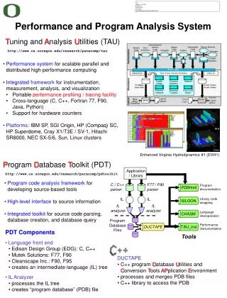
Scalable Deep Analytics on Cloud and High Performance Computing Environments

1. Scalable Deep Analytics on Cloud and High Performance Computing Environments Geoffrey Fox gcf@indiana.edu http://www.infomall.orghttp://www.futuregrid.org School of Informatics and Computing Digital Science Center Indiana University Bloomington NASA SACD Lecture Series on Complex Systems and Deep Analytics NASA Langley Research Center Building 1209, Room 180 Conference RoomAugust 8 2012

2. Abstract • We posit that big data implies  robust data-mining algorithms that must run in parallel to achieve needed performance. • Ability to use Cloud computing allows us to tap cheap commercial resources and several important data and programming advances. Nevertheless we also need to exploit traditional HPC environments. We discuss our approach to this challenge which involves Iterative MapReduce as an interoperable Cloud-HPC runtime. • We stress that the communication structure of data analytics is very different from classic parallel algorithms as one uses large collective operations (reductions or broadcasts) rather than the many small messages familiar from parallel particle dynamics and partial differential equation solvers. • One needs different runtime optimizations from those in typical MPI runtimes. • We describe our experience using deterministic annealing to build robust parallel algorithms for clustering, dimension reduction and hidden topic/context determination. • We suggest that a coordinated effort is needed to build quality scalable robust data mining libraries to enable big data analysis across many fields.

3. Clouds Grids and HPC

4. Science Computing Environments • Large Scale Supercomputers – Multicore nodes linked by high performance low latency network • Increasingly with GPU enhancement • Suitable for highly parallel simulations • High Throughput Systems such as European Grid Initiative EGI or Open Science Grid OSG typically aimed at pleasingly parallel jobs • Can use “cycle stealing” • Classic example is LHC data analysis • Grids federate resources as in EGI/OSG or enable convenient access to multiple backend systems including supercomputers • Portals make access convenient and • Workflow integrates multiple processes into a single job • Specialized visualization, shared memory parallelization etc. machines

5. Clouds and Grids/HPC • Synchronization/communication PerformanceGrids > Clouds > Classic HPC Systems • Clouds naturally execute effectively Grid workloads but are less clear for closely coupled HPC applications • Service Oriented Architectures portals and workflow appear to work similarly in both grids and clouds • May be for immediate future, science supported by a mixture of • Clouds – some practical differences between private and public clouds – size and software • High Throughput Systems (moving to clouds as convenient) • Grids for distributed data and access • Supercomputers (“MPI Engines”) going to exascale

6. What Applications work in Clouds • Pleasingly parallel applications of all sorts with roughly independent data or spawning independent simulations • Long tail of science and integration of distributed sensors • Commercial and Science Data analytics that can use MapReduce (some of such apps) or its iterative variants (mostother data analytics apps) • Which science applications are using clouds? • Many demonstrations –Conferences, OOI, HEP …. • Venus-C (Azure in Europe): 27 applications not using Scheduler, Workflow or MapReduce (except roll your own) • 50% of applications on FutureGrid are from Life Science but there is more computer science than total applications • Locally Lilly corporation is major commercial cloud user (for drug discovery) but Biology department is not

7. 2 Aspects of Cloud Computing: Infrastructure and Runtimes • Cloud infrastructure: outsourcing of servers, computing, data, file space, utility computing, etc.. • Cloud runtimes or Platform:tools to do data-parallel (and other) computations. Valid on Clouds and traditional clusters • Apache Hadoop, Google MapReduce, Microsoft Dryad, Bigtable, Chubby and others • MapReduce designed for information retrieval but is excellent for a wide range of science data analysis applications • Can also do much traditional parallel computing for data-mining if extended to support iterative operations • Data Parallel File system as in HDFS and Bigtable

8. Analytics and Parallel Computing on Clouds and HPC

9. Classic Parallel Computing • HPC: Typically SPMD (Single Program Multiple Data) “maps” typically processing particles or mesh points interspersed with multitude of low latency messages supported by specialized networks such as Infiniband and technologies like MPI • Often run large capability jobs with 100K (going to 1.5M) cores on same job • National DoE/NSF/NASA facilities run 100% utilization • Fault fragile and cannot tolerate “outlier maps” taking longer than others • Clouds: MapReduce has asynchronous maps typically processing data points with results saved to disk. Final reduce phase integrates results from different maps • Fault tolerant and does not require map synchronization • Map only useful special case • HPC + Clouds: Iterative MapReduce caches results between “MapReduce” steps and supports SPMD parallel computing with large messages as seen in parallel kernels (linear algebra) in clustering and other data mining

10. (b) Classic MapReduce (a) Map Only (c) Iterative MapReduce (d) Loosely Synchronous 4 Forms of MapReduce Pij Input Input Iterations Input Classic MPI PDE Solvers and particle dynamics BLAST Analysis Parametric sweep Pleasingly Parallel High Energy Physics (HEP) Histograms Distributed search Expectation maximization Clustering e.g. Kmeans Linear Algebra, Page Rank map map map MPI Exascale Domain of MapReduce and Iterative Extensions Science Clouds reduce reduce Output

11. Commercial “Web 2.0” Cloud Applications • Internet search, Social networking, e-commerce, cloud storage • These are larger systems than used in HPC with huge levels of parallelism coming from • Processing of lots of users or • An intrinsically parallel Tweet or Web search • Classic MapReduce is suitable (although Page Rank component of search is parallel linear algebra) • Data Intensive • Do not need microsecond messaging latency

12. Data Intensive Applications • Applications tend to be new and so can consider emerging technologies such as clouds • Do not have lots of small messages but rather large reduction (aka Collective) operations • New optimizations e.g. for huge messages • e.g. Expectation Maximization (EM) dominated by broadcasts and reductions • Not clearly a single exascale job but rather many smaller (but not sequential) jobs e.g. to analyze groups of sequences • Algorithms not clearly robust enough to analyze lots of data • Current standard algorithms such as those in R library not designed for big data • Our Experience • Multidimensional Scaling MDS is iterative rectangular matrix-matrix multiplication controlled by EM • Deterministically Annealed Pairwise Clustering as an EM example

13. Generalize to arbitrary Collective Twister for Data Intensive Iterative Applications Compute Communication Reduce/ barrier Broadcast • (Iterative) MapReduce structure with Map-Collective is framework • Twister runs on Linux or Azure • Twister4Azure is built on top of Azure tables, queues, storage New Iteration Smaller Loop-Variant Data Larger Loop-Invariant Data

14. Performance – Kmeans Clustering Overhead between iterations First iteration performs the initial data fetch Twister4Azure Task Execution Time Histogram Number of Executing Map Task Histogram Performance with/without data caching Speedup gained using data cache Hadoop Twister Hadoop on bare metal scales worst Twister4Azure(adjusted for C#/Java) Scaling speedup Strong Scaling with 128M Data Points Increasing number of iterations Weak Scaling Qiu, Gunarathne

15. Data Intensive Kmeans Clustering • ─ Image Classification: 1.5 TB; 500 features per image;10k clusters • 1000 Map tasks; 1GB data transfer per Map task Work of Qiu and Zhang

16. Broadcast Twister Communication Steps Map Tasks Map Tasks Map Tasks Broadcasting Data could be large Chain & MST Map Collectives Local merge Reduce Collectives Collect but no merge Combine Direct download or Gather Map Collective Map Collective Map Collective Reduce Tasks Reduce Tasks Reduce Tasks Reduce Collective Reduce Collective Reduce Collective Work of Qiu and Zhang Gather

17. Polymorphic Scatter-Allgather in Twister Work of Qiu and Zhang

18. Twister Performance on Kmeans Clustering Work of Qiu and Zhang

19. Data Analytics

20. General Remarks I • No agreement as to what is data analytics and what tools/computers needed • Databases or NOSQL? • Shared repositories or bring computing to data • What is repository architecture? • Data from observation or simulation • Data analysis, Datamining, Data analytics., machine learning, Information visualization • Computer Science, Statistics, Application Fields • Big data (cell phone interactions) v. Little data (Ethnography, surveys, interviews) • Provenance, Metadata, Data Management

21. General Remarks II • Regression analysis; biostatistics; neural nets; bayesian nets; support vector machines; classification; clustering; dimension reduction; artificial intelligence • Patient records growing fast • Abstract graphs from net leads to community detection • Some data in metric spaces; others very high dimension or none • Large Hadron Collider analysis mainly histogramming – all can be done with MapReduce • Google, Bing largest data analytics in world • Time Series from Earthquakes to Tweets to Stock Market • Pattern Informatics • Image Processing from climate simulations to NASA to DoD • Financial decision support; marketing; fraud detection; automatic preference detection (map users to books, films)

22. Data Data Data Data Traditional File System? • Typically a shared file system (Lustre, NFS …) used to support high performance computing • Big advantages in flexible computing on shared data but doesn’t “bring computing to data” • Object stores similar structure (separate data and compute) to this C C C C C C C C C C C C C C C S S S S Archive C Compute Cluster Storage Nodes

23. Data Data Data Data Data Data Data Data Data Data Data Data Data Data Data Data Data Parallel File System? Replicate each block Breakup • No archival storage and computing brought to data C C C C C C C C C C C C C C C C Block1 Block1 Block2 Block2 File1 File1 Replicate each block …… …… Breakup BlockN BlockN

24. Building High Level Tools • Automatic Layer Determination developed by David Crandall added to collaboration from the faculty at Indiana University • Hidden Markov Method based Layer Finding Algorithm. automatic layer finding algorithm manual method Data Browser

25. “Science of Science”TeraGridUser Areas

26. Science Impact Occurs Throughout the Branscomb Pyramid

30. Data Intensive Futures? • PETScandScaLAPACKand similar libraries very important in supporting parallel simulations • Need equivalent Data Analytics libraries • Include datamining (Clustering, SVM, HMM, Bayesian Nets …), image processing, information retrieval including hidden factor analysis (LDA), global inference, dimension reduction • Many libraries/toolkits (R, Matlab) and web sites (BLAST) but typically not aimed at scalable high performance algorithms • Should support clouds and HPC; MPI and MapReduce • Iterative MapReduce an interesting runtime; Hadoop has many limitations • Need a coordinated Academic Business Government Collaboration to build robust algorithms that scale well • Crosses Science, Business Network Science, Social Science • Propose to build community to define & implementSPIDAL or Scalable Parallel Interoperable Data Analytics Library

31. Deterministic Annealing

32. Some Motivation • Big Data requires high performance – achieve with parallel computing • Big Data requires robust algorithms as more opportunity to make mistakes • Deterministic annealing (DA) is one of better approaches to optimization • Tends to remove local optima • Addresses overfitting • Faster than simulated annealing • Return to my heritage (physics) with an approach I called Physical Computation (cf. also genetic algs) -- methods based on analogies to nature • Physics systems find true lowest energy state if you anneal i.e. you equilibrate at each temperature as you cool

33. Some Ideas • Deterministic annealing is better than many well-used optimization problems • Started as “Elastic Net” by Durbin for Travelling Salesman Problem TSP • Basic idea behind deterministic annealing is mean field approximation, which is also used in “Variational Bayes” and many “neural network approaches” • Markov chain Monte Carlo (MCMC) methods are roughly single temperature simulated annealing • Less sensitive to initial conditions • Avoid local optima • Not equivalent to trying random initial starts

34. Uses of Deterministic Annealing • Clustering • Vectors: Rose (Gurewitz and Fox) • Clusters with fixed sizes and no tails (Proteomics team at Broad) • No Vectors: Hofmann and Buhmann (Just use pairwise distances) • Dimension Reduction for visualization and analysis • Vectors: GTM • No vectors: MDS (Just use pairwise distances) • Can apply to HMM & general mixture models(less study) • Gaussian Mixture Models • Probabilistic Latent Semantic Analysis with Deterministic Annealing DA-PLSA as alternative to Latent Dirichlet Allocation applied to documents or file access classification

35. Basic Deterministic Annealing • Gibbs Distribution at Temperature TP() = exp( - H()/T) /  d exp( - H()/T) • Or P() = exp( - H()/T + F/T ) • Minimize Free Energy combining Objective Function and EntropyF= < H- T S(P) > =  d {P()H+ T P() lnP()} • H is objective function to be minimized as a function of parameters  • Simulated annealing corresponds to doing these integrals by Monte Carlo • Deterministic annealing corresponds to doing integrals analytically (by mean field approximation) and is much faster than Monte Carlo • In each case temperature is lowered slowly – say by a factor 0.95 to 0.99 at each iteration • I used 0.9998484 in recent case when finding 29000 clusters

36. Implementation of DA Central Clustering • Here points are in a metric space • Clustering variables are Mi(k) where this is probability that point ibelongs to cluster k andk=1KMi(k) = 1 • In Central or PW Clustering, take H0 = i=1Nk=1K Mi(k) i(k) • Linear form allows DA integrals to be done analytically • Central clustering hasi(k) = (X(i)- Y(k))2 and Mi(k) determined by Expectation step • HCentral = i=1Nk=1KMi(k) (X(i)- Y(k))2 • <Mi(k)> = exp( -i(k)/T ) / k=1Kexp( -i(k)/T ) • Centers Y(k) are determined in M step of EM method

37. DeterministicAnnealing • Minimum evolving as temperature decreases • Movement at fixed temperature going to false minima if not initialized “correctly F({y}, T) Solve Linear Equations for each temperature Nonlinear effects mitigated by initializing with solution at previous higher temperature Configuration {y}

38. Rose, K., Gurewitz, E., and Fox, G. C. ``Statistical mechanics and phase transitions in clustering,'' Physical Review Letters, 65(8):945-948, August 1990. My #6 most cited article (424 citesincluding 14 in 2012) • System becomes unstable as Temperature lowered and there is a phase transition and one splits cluster into two and continues EM iteration • One can start with just one cluster

39. General Features of DA • Deterministic Annealing DA is related to Variational Inference or Variational Bayes methods • In many problems, decreasing temperature is classic multiscale – finer resolution (√T is “just” distance scale) • We have factors like (X(i)- Y(k))2/ T • In clustering, one then looks at second derivative matrix of FR (P0) wrtand as temperature is lowered this develops negative eigenvalue corresponding to instability • Or have multiple clusters at each center and perturb • This is a phase transition and one splits cluster into two and continues EM iteration • One can start with just one cluster

40. Start at T= “” with 1 Cluster • Decrease T, Clusters emerge at instabilities

43. Some non-DA Ideas • Dimension reduction gives Low dimension mappings of data to both visualize and apply geometric hashing • No-vector (can’t define metric space) problems are O(N2) • Genes are no-vector unless multiply aligned • For no-vector case, one can develop O(N) or O(NlogN) methods as in “Fast Multipole and OctTree methods” • Map high dimensional data to 3D and use classic methods developed originally to speed up O(N2) 3D particle dynamics problems

44. General Deterministic Annealing • For some cases such as vector clustering and Mixture Models one can do integrals by hand but usually that will be impossible • So introduce Hamiltonian H0(, ) which by choice of can be made similar to real Hamiltonian HR() and which has tractable integrals • P0() = exp( - H0()/T + F0/T ) approximate Gibbs for HR • FR (P0) = < HR - T S0(P0) >|0 = < HR – H0> |0 + F0(P0) • Where <…>|0 denotes  d Po() • Easy to show that real Free Energy (the Gibb’s inequality)FR (PR) ≤ FR (P0) (Kullback-Leibler divergence) • Expectation step E is find  minimizing FR (P0) and • Follow with M step (of EM) setting  = <> |0 =  dPo() (mean field) and one follows with a traditional minimization of remaining parameters Note 3 types of variablesused to approximate real Hamiltonian subject to annealing The rest – optimized by traditional methods

45. Implementation of DA-PWC • Clustering variables are again Mi(k) (these are  in general approach) where this is probability point ibelongs to cluster k • Pairwise Clustering Hamiltonian given by nonlinear form • HPWC= 0.5 i=1Nj=1N(i, j) k=1KMi(k) Mj(k) / C(k) • (i, j) is pairwise distance between points i and j • with C(k) = i=1NMi(k) as number of points in Cluster k • Take same form H0 = i=1Nk=1K Mi(k) i(k) as for central clustering • i(k) determined to minimize FPWC (P0) = < HPWC - T S0(P0) >|0where integrals can be easily done • And now linear (in Mi(k)) H0 and quadratic HPC are different • Again <Mi(k)> = exp( -i(k)/T ) / k=1Kexp( -i(k)/T )

46. Continuous Clustering • This is a subtlety introduced by Ken Rose but not widely known • Take a cluster k and split into 2 with centers Y(k)A and Y(k)B with initial valuesY(k)A = Y(k)B at original center Y(k) • Then typically if you make this change and perturb the Y(k)AY(k)B, they will return to starting position as F at stable minimum • But instability can develop and one finds • Implement by adding arbitrary number p(k) of centers for each cluster Zi = k=1K p(k) exp(-i(k)/T) and M step gives p(k) = C(k)/N • Halve p(k) at splits; can’t split easily in standard case p(k) = 1 Free Energy F Y(k)A and Y(k)B Free Energy F Free Energy F Y(k)A- Y(k)B Y(k)A+ Y(k)B

47. Trimmed Clustering(“Sponge Vector”)Deterministic Annealing

48. Trimmed Clustering • Clustering with position-specific constraints on variance: Applying redescending M-estimators to label-free LC-MS data analysis (Rudolf Frühwirth, D R Mani and SaumyadiptaPyne) BMC Bioinformatics 2011, 12:358 • HTCC= k=0Ki=1NMi(k) f(i,k) • f(i,k) = (X(i) - Y(k))2/2(k)2 k > 0 • f(i,0) = c2 / 2 k = 0 • The 0’th cluster captures (at zero temperature) all points outside clusters (background) • Clusters are trimmed (X(i) - Y(k))2/2(k)2< c2 / 2 • Applied toProteomics Mass Spectrometry T = 1 T ~ 0 T = 5 Distance from cluster center

49. Proteomics 2D DA Clustering Sponge Peaks Centers

50. Introduce Sponge Running on 8 nodes, 16 cores each 241605 Peaks Complex Parallelization of Peaks=points (usual) andClusters (Switch on after # gets large) High Temperature -- Start Low Temperature -- End