Download
1 / 28
280 likes | 358 Views
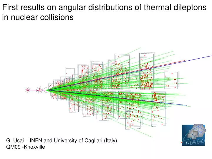
First results on angular distributions of thermal dileptons in nuclear collisions. G. Usai – INFN and University of Cagliari (Italy) QM09 -Knoxville. Summary of previous results on thermal dileptons. Phys. Rev. Lett. 96 (2006) 162302.

E N D
First results on angular distributions of thermal dileptons in nuclear collisions G. Usai – INFN and University of Cagliari (Italy) QM09 -Knoxville
Summary of previous results on thermal dileptons Phys. Rev. Lett. 96 (2006) 162302 • Invariant mass region M<1 GeV: thermal dilepton production largely mediated by the broad vector meson ρ viapp→r→g→mmannihilation. Hadronic nature supported by the rise of radial flow up to M=1 GeV • M>1 GeV: sudden fall of radial flow of thermal dimuons occurs , naturally explained as a transition to a qualitatively different source, i.e.mostly partonicradiation,qq→g→μμ Phys. Rev. Lett. 100 (2008) 022302 2
Is the radiation thermal? Features of thermal radiation: - Plack-like exponential shape of mass spectra (for flat spectral function) - mT scaling of transverse momentum spectra - Absence of any polarization in angular distributions (this talk) - Agreement between data and thermal models in yields and spectral shapes
Excess mass spectrum up to 2.5 GeV All known sources (hadro-cocktail, open charm, DY) subtracted Acceptance corrected spectrum (pT>0.2 GeV) Absolute normalization → comparison to theory in absolute terms! thermalpp g mm(M<1 GeV) && thermalqq g mm(M >1 GeV) suggested dominant by Teff vs M (supported by R/R, D/Z) also multipion processes (H/R) Eur. Phys. J. C 59 (2009) 607 Planck-like mass spectrum; falling exponentially Agreement with theoretical models up to 2.5 GeV! 4
Angular distributions General formalism for the description of an angular distribution dσ/dcosθ df is the differential decay angular distribution in the rest frame of the virtual photon g* with respect to a suitably chosen axis l, m,n are structure functions related to helicity structure functions and the spin density matrix elements of the virtual photon 5
What can we learn from angular distributions? Analysis in the mass region M<1 GeV: excess dileptons produced from annihilation of pions However, pions are spinless: Don’t we expect to find a trivial result for λ, μ and ν? The answer is no! Even for annihilation of spinless particles, like pp annihilation, the structure function parameters can have any value λ, μ, ν ǂ 0 for collinear pions along z axis l = -1 longitudinal polarization of the virtual photon However, a completely random orientation of annihilating pions in 3 dimensions would lead to l, m, n = 0 6
y x pµ+ CS z axis pprojectile ptarget Viewed from dimuonrest frame Reference frame Collins Soper (CS) frame θ is the angle between the positive muon pμ+ and the z-axis. The z axis is the bisector between pproj and - ptarget ϕ Choice of the frame non relevant: once all measured, l, m, n can be re-computed in any other frame with a simple transformation (Z. Phys. C31, 513 (1986)) 7
Angular distributions in the low mass region • Results on centrality integrated data with pT>0.6 GeV for: • Excess dileptons in 2 mass windows: • 0.4<M<0.6 GeV (~17600 mm pairs) 0.6<M<0.9 GeV (~36000 mm pairs) • Vector mesons ω and f (~73000 mm pairs) 8
Analysis steps Analysis done in cosθ-f space with different binnings in [dN/dcosθdf]m x nto study the systematics • Steps followed for each of the [m x n] bins: • Combinatorial background subtraction • 2) Assessment of fake matches • 3) Isolation of excess by subtraction of the known sources • Acceptance correction in 2-dim cosθ-f space or in 1-dim projections
Combinatorial background subtraction Combinatorial background reduced for pT>0.6 GeV: B/S ~ 2-3 Systematic errors due to subtraction of combinatorial background ~2-3% Example: 0.0<IcosθI<0.1 and 4 bins in IcosfI checked in all other bins 10
Overlay Monte Carlo: Monte Carlo muons superimposed to real events and reconstructed Fake matches are tagged and the relative fraction of correct matched muons is evaluated Systematic errors due to subtraction of fakes <1% Muon spectrometer muon trigger and tracking fake target Fake match: muon matched to a wrong track in the vertex telescope Can be important in high multiplicity events (negligible in pA or peripheral AA) Hadron absorber correct hadron absorber Assessment of fake matches 11
Subtraction of known sources Systematic uncertainties: 4-6% - up to 10-15% in some low-populated cosθ-f bins →main source of systematic errors However, measurement still dominated by statistical errors 12
Acceptance correction Acceptance projections in IcosθI and If I 1-dim correction: full range in cosθ and f used 2-dim correction: 0.7<|f|<2.4 (-0 .75<cosf <0.75) applied to exclude regions with very low acceptance 13
Acceptance corrected decay angular distributions Final results on acceptance corrected f meson Excess 0.6<M<0.9 GeV 14
Determination of the structure coefficients I Three methods Method 1: Analysis of the 2-dim distribution cosθ-cosf restricted to 6x6 matrix -0.6<cosθ<0.6 (bin width 0.2) -0 .75<cosf <0.75 (bin width 0.25) Fit with function to extract all 3 structure parameters
Determination of the structure coefficients II Method 2: Project 2-dim decay angular distribution over polar or azimuth angle |cosθ|<0.8 (bin width 0.1) |cosf |<0.75 (bin width 0.25) Fit over polar angle Fit over azimuth angle Method 3: Analysis of the inclusive distributions in |cosθ| and |f | with a 1-dim acceptance correction |cosθ|<0.8 (bin width 0.1) 0<IfI<p (bin width 0.3) Analysis of projections: m fixed to value found from method 1
Structure coefficients l,m,n: excess 0.6<M<0.9 GeV Method 1:2-dim fit to data with Results: l = -0.19 ± 0.12 n = 0.03 ± 0.15 μ = 0.05 ± 0.03 All parameters zero within errors 17
Structure coefficients l,m,n: excess 0.4<M<0.6 GeV Method 1:2-dim fit to data with Results l = -0.13 ± 0.27 n = 0.12 ± 0.30 μ = -0.04 ± 0.10 All parameters zero within errors 18
Structure coefficients l,m,n: ω and ɸ mesons Method 1:2-dim fit to data with Results for the ω l = -0.10 ± 0.10 n = 0.05 ± 0.11 μ = -0.05 ± 0.02 Results for the f l = -0.07 ± 0.09 n = -0.10 ± 0.08 μ = 0.04 ± 0.02 All parameters zero within errors 19
Polar angular distributions: excess Method 2: Fix m = 0 and project the decay angular distribution over polar or azimuth angles Submitted to PRL, arXiv:0812.3100 excess (0.6<M<0.9 GeV) Fit function for polar angle l=-0.13±0.12 (n= 0.05±0.15) Fit function for azimuth angle excess (0.4<M<0.6 GeV) Uniform polar distributions : no polarization for the excess in the ρ like region 0.6<M<0.9 GeV and in the region 0.4<M<0.6 GeV l=-0.10±0.24 (n=0.11 ±0.30)
Polar angular distributions: and f Submitted to PRL, arXiv:0812.3100 Method 2: Fix m = 0 and project the decay angular distribution over polar or azimuth angles meson Fit function for polar angle l=-0.12±0.09 (n=-0.06±0.10) Fit function for azimuth angle fmeson Uniform polar distributions : no polarization also for ω and f l=-0.13±0.08 (n=-0.09±0.08)
Azimuth angular distributions: excess Submitted to PRL, arXiv:0812.3100 Method 3: Fix m = 0 -analysis of the inclusive distributions in |cosθ| and | f| with 1-dim acceptance correction excess (0.6<M<0.9 GeV) n=0.00±0.12 (l=-0.15±0.09) Fit function for polar angle Fit function for azimuth angle excess (0.4<M<0.6 GeV) Uniform azimuth distributions for the excess in the ρ like region 0.6<M<0.9 GeV and in the region 0.4<M<0.6 GeV n=0.10±0.18 (l=-0.09±0.16) 22
Azimuth angular distributions: and f Submitted to PRL, arXiv:0812.3100 Method 3: Fix m = 0 -analysis of the inclusive distributions in |cosθ| and | f| with 1-dim acceptance correction meson n=-0.02±0.08 (l=-0.12±0.06) Fit function for polar angle Fit function for azimuth angle fmeson n=-0.06±0.06 (l=--0.05±0.06) Uniform azimuth distributions also for ω and f
Comparison of results from different methods Choice of the frame non relevant: once all measured, l, m, n can be re-computed in any other frame with a simple transformation (Z. Phys. C31, 513 (1986)) → l, m, n re-computed in Gottfried-Jackson frame l, m, n zero also in Gottfried-Jackson frame
Summary Absence of any polarization: Fully consistent with the interpretation of the observed excess as thermal radiation Necessary but not sufficient condition Put together with other features: Planck-like shape of mass spectra, temperature systematics, agreement of data with thermal models Thermal interpretation more plausible than ever before
Pure in-medium part M>1 GeV: sudden fall of radial flow of thermal dimuons occurs , naturally explained as a transition to a qualitatively different source, i.e.mostly partonicradiation,qq→g→μμ HADRONIC source alone (2pi+4pi+a1pi)(in HYDRO and other models of fireball expansion) continuous rise of Teff with mass, no way to get a discontinuity at M=1 GeV like at any other mass value Uncertainty in fraction of QGP, 50%, 60%, 80%, …. But a strong contribution of partonic source is needed to get a discontinuity in Teff at M=1GeV, HADRONIC source ALONE CANNOT do that 27 27