Download
1 / 25
260 likes | 388 Views
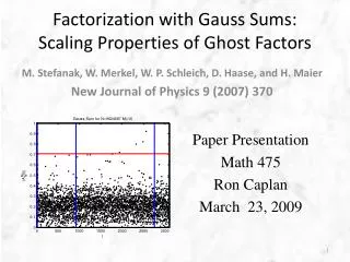
Factorization with Gauss Sums: Scaling Properties of Ghost Factors. Paper Presentation Math 475 Ron Caplan March 23, 2009. M. Stefanak , W. Merkel, W. P. Schleich , D. Haase , and H. Maier New Journal of Physics 9 (2007) 370. Outline. Introduction

E N D
Factorization with Gauss Sums: Scaling Properties of Ghost Factors Paper Presentation Math 475 Ron Caplan March 23, 2009 M. Stefanak, W. Merkel, W. P. Schleich, D. Haase, and H. Maier New Journal of Physics 9 (2007) 370
Outline • Introduction • Factoring with Gauss Sums: Ghost Factors • 4 Classes of Trial Factors • Truncation Parameter for Complete Suppression of Ghost Factors • Scaling of Ghost Factors with Counting Function • Uniform distribution of fractional part • Non-uniform distribution of fractional part • Optimal scaling law • Summery of Results • Friendly Ghost Factors? • Conclusion
Introduction • Gauss sums are prevalent in descriptions of various physical systems including optics and quantum mechanics. • Can be used to factor large numbers, an important task for cryptography etc. • Full vs. Truncated: Lower number of terms in sum better for experiments, but ghost factors appear. • Want to know how ghost factors scale with number of summation terms, to find min terms necessary
Factoring with Gauss Sums Complete Gauss Sum: Total # of Terms to Sum: Example:
Factoring with Gauss Sums Total # of Terms to Sum: Truncated Gauss Sum: Ghosts! Example:
Classification of Trial Factors • Actual factors – constant value of 1 for all M • Non-factors that decay quickly with higher M • Ghost factors which require large M to decay • Threshold non-factors that do not decay with larger M • Even integer • Close to odd integer • Close to even integer • Midpoint between even and odd integer
New Form for Gauss Sum • Since 2N/l determines the class of trial factors, useful to re-write the Gauss sum Define normalized curlicue function: Fractional part: Can now write Gauss sum as: corresponds to factors, close to 0, to ghost factors. is even about tau because:
New Form of Gauss Sum For large M: Define: of N is
Threshold Values Factors
Truncation Parameter • Need to determine truncation parameter that will suppress all ghost factors below threshold • Since ghost factors occur for very small values of we can replace summation with an approximate integral Note Substitute: Fresnel integral:
Truncation Parameter Black: Discrete Red: Fresnel Int Approx
Truncation Parameter sol of Natural threshold: Minimum value at largest l: (numeric) Scaling unchanged by threshold value – only pre-factor changes!
Ghost Factor Counting • Have found sufficient condition to suppress ghosts • Now, want to find necessary condition Ghost factor counting function:
Ghost Factor Counting Ghost factors occur in region of s: From Fresnel: Total width of s with values larger than : Now want to relate g(N.M) to width via distribution of for a given N 2 Cases: Uniform Distribution Non-uniform Distribution
Ghost Factor Counting Uniform Distribution Remember: So # of ghosts directly proportional to width: Inverse power law Example: M = ln N:
Ghost Factor Counting 10,000 random numbers from M = ln N Non-uniform distribution!
Ghost Factor Counting Non-uniform Distribution Happens when N has few divisors, but nearby number N+k has many. Example:
Ghost Factor Counting Non-uniform Distribution l’ data points (factors of N’) in interference pattern of N follow curve: Tends to 0 for large l’, so becomes ghost factor:
Optimality of 4th root Law Remember for uniform distribution we have: Non-uniform: Uniform: Faster than uniform:
Optimality of 4th root Law Idea! Since g(N.M) decays fast at first, why not allow K ghosts: Only used uniform distribution, non-uniform cases, Mk may even be larger! Compare with: So, even if we tolerate K ghosts, we cannot do better then a scaling for required M So, 4th root scaling is both sufficient and necessary!
Results To eliminate all ghost factors for ANY N, need: Number of terms to sum: Full Gauss sum requires terms, so we save a bit [For some N, need less M … what percentages?] Are ghost factors really that bad? …………
Results: Friendly Ghost Factors We now know that ghost factors are actually real factors of a nearby number N + k May be possible to exploit this fact to factor numbers more efficiently M=17 not good to suppress ghosts, but we can fit them to curves of factors of different N-primes Can possibly come up with new scheme taking advantage of this…(?)
Conclusion • Ghost factors are factors of neighboring numbers • Using 4th root law, can eliminate all ghost factors Outlook • Ghost factors may be helpful in forming new algorithms to factor numbers. • Some experiments (like BEC diffraction) seem to compute higher power Gauss sums (like cubic) which can help the scaling for M0.