Download
1 / 10
110 likes | 203 Views
Count Data. Harry R. Erwin, PhD School of Computing and Technology University of Sunderland. Resources. Crawley, MJ (2005) Statistics: An Introduction Using R. Wiley. Freund, RJ, and WJ Wilson (1998) Regression Analysis, Academic Press.

E N D
Count Data Harry R. Erwin, PhD School of Computing and Technology University of Sunderland
Resources • Crawley, MJ (2005) Statistics: An Introduction Using R. Wiley. • Freund, RJ, and WJ Wilson (1998) Regression Analysis, Academic Press. • Gentle, JE (2002) Elements of Computational Statistics. Springer. • Gonick, L., and Woollcott Smith (1993) A Cartoon Guide to Statistics. HarperResource (for fun).
Introduction • These four demonstration sessions of this class address special types of data: • Counts • Proportions • Survival analysis • Binary responses
Frequencies and Proportions • With frequency data, we know how often something happened, but not how often it didn’t happen. • With proportion data (next week), we know how often it didn’t happen.
Count Data • Linear regression assumes constant variance and normal errors. This is not appropriate for count data: • Counts are non-negative. • Response variance usually increases with the mean. • Errors are not normally distributed. • Zeros are hard to transform.
Handling Count Data in R • Use a glmwith family=poisson. • This sets errors to Poisson, so variance is proportional to the mean. • This sets link to log, so fitted values are positive. • Book example • If you have overdispersion (residual deviance greater than residual degrees of freedom), use family=quasipoisson.
Analysis of Count Data • Book example (230ff) • Use of table() • Use of tapply() • fitting the glm with family = poisson. • refitting with family = quasipoisson. • three and four-way interactions • model simplification • documentation
Contingency Tables • Risk of data aggregation over important explanatory variables (nuisance variables) • Book example (234ff) • The saturated model • Remove the N-way interaction and see if it was significant. • If the N-way interaction is significant, go no further. • Then remove the scientifically interesting interaction and see if it is significant. • You have to check the nuisance variables first!
ANCOVA with Counts • Book example (237ff) • plotting and use of split to gain insight. • analysis—testing for the need for different slopes. • use of predict() to draw lines through the plot.
Frequency Distributions • Book example (240ff) • testing for independence • use of table() • use of dpois() • plotting and interpretation • use the negative binomial distribution for data with variance much greater than the mean • use the binomial distribution for data with variance less than the mean