NECSI Summer School 2008 Week 3: Methods for the Study of Complex Systems Stochastic Systems

1. NECSI Summer School 2008Week 3: Methods for the Study of Complex SystemsStochastic Systems Hiroki Sayama sayama@binghamton.edu

2. Four approaches to complexity Nonlinear Dynamics Complexity = No closed-form solution, Chaos Information Complexity = Length of description, Entropy Computation Complexity = Computational time/space, Algorithmic complexity Collective Behavior Complexity = Multi-scale patterns, Emergence

3. Stochastic system • Deterministic system xt = F(xt-1, t) • Stochastic system (w/ discrete states) Px(s; t) = Ss’ Px(s|s’) Px(s’; t-1) Px(s; t): Probability for x to be s at time t Px(s|s’): Transition probability for x in state s’ to change to s in one time step • Assumed time-independent

4. 1/4 0 1 3/4 3/4 1/4 Exercise • Write the model of the following system in mathematical form • Numbers on arrows are transition probabilities

5. Random Walk

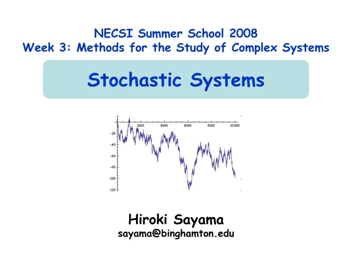
6. Random walk • Time series in which random noise is added to the system’s previous state xt = xt-1 + d • d : random variable (e.g., +1 or -1) • Many stochastic events that accumulate and form the system’s history

7. Exercise • Derive a mathematical representation of random walk using probability distribution, assuming: • Possible states: integers (unbounded) • Probability of moving upward and downward: 50%-50% Px(s|s’) = ½ d(s, s’+1) + ½ d(s, s’-1) d(a,b): Kronecker’s delta function

8. Where will you be after t steps? • Exact position of individual random walk is hard to predict, but you can still statistically describe where itis likely to go

9. Exercise • Show analytically that the expected position of a particle in random walk will not change over time <s> = Ss s Px(s; t)

10. Exercise • Show analytically that the root square means (RMS) distance a particle travels in random walk will grow over time with power=1/2 √<(s-s0)2> = { Ss (s-s0)2 Px(s; t) }1/2

11. Dependence on time scale • Distribution of positions flattens over time (diffusion of probability)

12. After sufficiently long time • Positions of many random-walking particles follow a “normal distribution” • A.k.a. Gaussian distribution, bell curve ~ e-(x-m)2/(2s2)/(2ps2)1/2 m: mean s: standard deviation s m

13. Relation to the central limit theorem • Sum (and hence average) of many independent random events will approximately follow a normal distribution (regardless of probability distribution of those random events) • Each step of random walk corresponds to an independent event • Position of a particle corresponds to the sum of those events

14. Self-Similar Properties of Individual Random Walk

15. Structure of a single random walk Random walk produces self-similar trajectory

16. Fractal time series • Random walk is a very simple example of “fractal” time series • Time series whose portionhas statistical properties similar to those of the whole series itself • Shows stochastic self-similarity • The word “fractal” came from the fact that these structures have fractional (non-integral) dimensions

17. Power of large fluctuation Power of small fluctuation The more data you collect, the larger fluctuation you find (scaling) Power law (scaling law) P P(w) ~ w-k • Random walk’s power spectrum shows an inverse power law distribution • For such systems, averaging system states over time fails w

18. Exercise: Failure of averaging • Produce time series data using a random walk model • Average the system state for the first t steps • Plot this average as a function of t • Does the average become more accurate as you increase t?

19. Dynamics of fractal time series • They are always fluctuating, but not completely random • There are gentle correlations between past, present, and future (regularity) • The similar dynamics appear over a wide range of time scales, without any characteristic frequency

20. Fractal time series in society • Many other real-world time series generated by complex social/ economical systems (i.e., many interacting parts) have fractal characteristics • Stock prices • Currency exchange rates

21. Fractal time series in biology • Many biological/physiological time series data are found to be fractal • Heartbeat rates, breathing intervals, human gaits, body temperature, etc. • They are usually fractal if a subject is normal and healthy • If they look very regular, the subject is probably not healthy • For details see, e.g., http://www.physionet.org/tutorials/fmnc/

22. Transition Probability Matrix and Asymptotic Probability Distribution

23. Time evolution of probabilities • If we consider probability distribution Px(si; t) as a meta-state of the system, its time evolution is linear Px(si; t) = Sj Px(si|sj) Px(sj; t-1) pt = A pt-1 • pt: Probability vector • A: Transition probability matrix • If original state space is finite and discrete

24. Convenient properties of transition probability matrix • The product of two TPMs is also a TPM • All TPMs have eigenvalue 1 • |l|  1 for all eigenvalues of any TPM • If the transition network is strongly connected, the TPM has one and only one eigenvalue 1 (no degeneration)

25. Exercise: Prove the following • The product of two TPMs is also a TPM • All TPMs have eigenvalue 1 • |l|  1 for all eigenvalues of any TPM • If the transition network is strongly connected, the TPM has one and only one eigenvalue 1 (no degeneration)

26. Answer (1) • All TPMs have eigenvalue 1 • You can show that there exists a non-zero vector q that satisfies A q = q, i.e. (A-I) q = 0 → |A-I| = 0 This holds when column vectors of A-I are linearly dependent with each other (i.e., A-I maps vectors to a subspace of fewer dimensions)

27. Answer (1) • A-I actually looks like this: • Note that each column vector is in a subspace s1+s2+...+sn = 0 → |A-I| = 0

28. Answer (2) • |l|  1 for all eigenvalues of any TPM • For any l, Amq = lmq (q: eigenvector) • Am is a product of TPM, therefore it must be a TPM as well whose elements are all <= 1 • Amq = lmq can’t diverge → |l|  1

29. TPM and asymptotic probability distribution • |l|  1 for all eigenvalues of any TPM • If the transition network is strongly connected, the TPM has one and only one eigenvalue 1 (no degeneration) → This eigenvalue is a unique dominant eigenvalue and the probability vector will eventually converge to its corresponding eigenvector

30. An Application:Google’s “PageRank”

31. ’s “PageRank” PageRank Explained (from http://www.google.com/technology/) “PageRank relies on the uniquely democratic nature of the web by using its vast link structure as an indicator of an individual page's value. In essence, Google interprets a link from page A to page B as a vote, by page A, for page B. But, Google looks at more than the sheer volume of votes, or links a page receives;it also analyzes the page that casts the vote. Votes cast by pages that are themselves "important" weigh more heavily and help to make other pages “important.” ”

32. PageRank explained mathematically • Lawrence Page, Sergey Brin, Rajeev Motwani, Terry Winograd, 'The PageRank Citation Ranking: Bringing Order to the Web' (1998): http://www-db.stanford.edu/~backrub/pageranksub.ps • Node: Web pages • link: WWW hyperlinks • State: Temporary “importance” of that node • Its coefficient matrix is atransition probability matrixthat can be obtained by dividing each column of the adjacency matrix by the number of 1’s in that column.

33. 0 0.5 0 0 1 0 0 0 0.5 0 1 0.5 0 0 0 0 0 0.5 0 0 0 0 0.5 0.5 0 Example (In the actual implementation of PageRank, positive non-zero weights are forcedly assigned to all pairs of nodes in order to make the entire network strongly connected) s1 s2 s5 s3 s4

34. Interpreting the PageRank network as a stochastic system (1) • State of each node can be viewed as a relative population that are visiting the webpage at t • At next timestep, the population will distribute to other webpages linked from that page evenly s1 s2 s5 s3 s4

35. Interpreting the PageRank network as a stochastic system (2) • Importance of each webpage can be measured by calculating the final equilibrium state of such population distribution s1 s2 s5 s3 s4

36. Therefore... • Just one dominant eigenvector of the TPM of a strongly connected network always exists, with l = 1 • This shows the equilibrium distribution of the population over WWW • So, just solvex = Axand you will get the PageRank for all the web pages on the World Wide Web!!

37. 0 0.5 0 0 1 0 0 0 0.5 0 1 0.5 0 0 0 0 0 0.5 0 0 0 0 0.5 0.5 0 Exercise Calculate the PageRank of each node in the above network (the network is already strongly connected so you can directly calculate its dominant eigenvector) s1 s2 s5 s3 s4

38. Summary • Stochastic systems may be modeled using probability distributions • Random walk shows ~t1/2 RMS growth and fractal time series patterns • Time evolution of probability distributions may be modeled and analyzed as a linear system • Asymptotic distribution can be uniquely obtained if the transition network is strongly connected

39. FYI: Master equation • A continuous-time analog of the same stochastic processes dP(s)/dt = Ss’≠s ( R(s|s’) P(s’) – R(s’|s) P(s) ) • R(a|b): Rate of transition from b to a