Download
1 / 38
390 likes | 486 Views
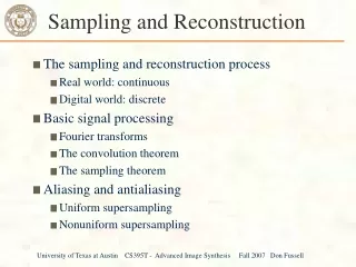
Sampling and Reconstruction. Reading. Required: Watt, Section 14.1 Recommended: Ron Bracewell, The Fourier Transform and Its Applications, McGraw-Hill.

E N D
Sampling and Reconstruction University of Texas at Austin CS384G - Computer Graphics Fall 2008 Don Fussell
Reading • Required: • Watt, Section 14.1 • Recommended: • Ron Bracewell, The Fourier Transform and Its Applications, McGraw-Hill. • Don P. Mitchell and Arun N. Netravali,“Reconstruction Filters in ComputerComputer Graphics ,” Computer Graphics, (Proceedings of SIGGRAPH 88). 22 (4), pp. 221-228, 1988. University of Texas at Austin CS384G - Computer Graphics Fall 2008 Don Fussell
What is an image? • We can think of an image as a function, f, from R2 to R: • f( x, y ) gives the intensity of a channel at position ( x, y ) • Realistically, we expect the image only to be defined over a rectangle, with a finite range: f: [a,b]x[c,d] [0,1] • A color image is just three functions pasted together. We can write this as a “vector-valued” function: • We’ll focus in grayscale (scalar-valued) images for now. University of Texas at Austin CS384G - Computer Graphics Fall 2008 Don Fussell
Images as functions University of Texas at Austin CS384G - Computer Graphics Fall 2008 Don Fussell
Digital images • In computer graphics, we usually create or operate on digital (discrete)images: • Sample the space on a regular grid • Quantize each sample (round to nearest integer) • If our samples are D apart, we can write this as: f[i ,j] = Quantize{ f(iD, jD) } University of Texas at Austin CS384G - Computer Graphics Fall 2008 Don Fussell
Motivation: filtering and resizing • What if we now want to: • smooth an image? • sharpen an image? • enlarge an image? • shrink an image? • Before we try these operations, it’s helpful to think about images in a more mathematical way… University of Texas at Austin CS384G - Computer Graphics Fall 2008 Don Fussell
Spatial domain Frequency domain Fourier transforms • We can represent a function as a linear combination (weighted sum) of sines and cosines. • We can think of a function in two complementary ways: • Spatially in the spatial domain • Spectrally in the frequency domain • The Fourier transform and its inverse convert between these two domains: University of Texas at Austin CS384G - Computer Graphics Fall 2008 Don Fussell
Spatial domain Frequency domain Fourier transforms (cont’d) • Where do the sines and cosines come in? • f(x) is usually a real signal, but F(s) is generally complex: • If f(x) is symmetric, i.e., f(x) = f(-x)), then F(s) = Re(s). Why? University of Texas at Austin CS384G - Computer Graphics Fall 2008 Don Fussell
1D Fourier examples University of Texas at Austin CS384G - Computer Graphics Fall 2008 Don Fussell
Spatial domain Frequency domain 2D Fourier transform Spatial domain Frequency domain University of Texas at Austin CS384G - Computer Graphics Fall 2008 Don Fussell
2D Fourier examples Frequency domain Spatial domain University of Texas at Austin CS384G - Computer Graphics Fall 2008 Don Fussell
Convolution • One of the most common methods for filtering a function is called convolution. • In 1D, convolution is defined as: where University of Texas at Austin CS384G - Computer Graphics Fall 2008 Don Fussell
Convolution properties • Convolution exhibits a number of basic, but important properties. • Commutativity: • Associativity: • Linearity: University of Texas at Austin CS384G - Computer Graphics Fall 2008 Don Fussell
= * f(x,y) h(x,y) g(x,y) Convolution in 2D • In two dimensions, convolution becomes: where University of Texas at Austin CS384G - Computer Graphics Fall 2008 Don Fussell
Convolution theorems • Convolution theorem: Convolution in the spatial domain is equivalent to multiplication in the frequency domain. • Symmetric theorem: Convolution in the frequency domain is equivalent to multiplication in the spatial domain. University of Texas at Austin CS384G - Computer Graphics Fall 2008 Don Fussell
Convolution theorems Theorem Proof (1) University of Texas at Austin CS384G - Computer Graphics Fall 2008 Don Fussell
1D convolution theorem example University of Texas at Austin CS384G - Computer Graphics Fall 2008 Don Fussell
2D convolution theorem example |F(sx,sy)| f(x,y) * h(x,y) |H(sx,sy)| g(x,y) |G(sx,sy)| University of Texas at Austin CS384G - Computer Graphics Fall 2008 Don Fussell
The delta function • The Dirac delta function, d(x), is a handy tool for sampling theory. • It has zero width, infinite height, and unit area. • It is usually drawn as: University of Texas at Austin CS384G - Computer Graphics Fall 2008 Don Fussell
Sifting and shifting • For sampling, the delta function has two important properties. • Sifting: • Shifting: University of Texas at Austin CS384G - Computer Graphics Fall 2008 Don Fussell
The shah/comb function • A string of delta functions is the key to sampling. The resulting function is called the shah or comb function: • which looks like: • Amazingly, the Fourier transform of the shah function takes the same form: where so = 1/T. University of Texas at Austin CS384G - Computer Graphics Fall 2008 Don Fussell
Sampling • Now, we can talk about sampling. • The Fourier spectrum gets replicated by spatial sampling! • How do we recover the signal? University of Texas at Austin CS384G - Computer Graphics Fall 2008 Don Fussell
Sampling and reconstruction University of Texas at Austin CS384G - Computer Graphics Fall 2008 Don Fussell
Sampling and reconstruction in 2D University of Texas at Austin CS384G - Computer Graphics Fall 2008 Don Fussell
Sampling theorem • This result is known as the Sampling Theorem and is generally attributed to Claude Shannon (who discovered it in 1949) but was discovered earlier, independently by at least 4 others: A signal can be reconstructed from its samples without loss of information, if the original signal has no energy in frequencies at or above ½ the sampling frequency. • For a given bandlimited function, the minimum rate at which it must be sampled is the Nyquist frequency. University of Texas at Austin CS384G - Computer Graphics Fall 2008 Don Fussell
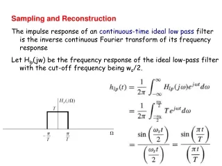
Reconstruction filters • The sinc filter, while “ideal”, has two drawbacks: • It has large support (slow to compute) • It introduces ringing in practice • We can choose from many other filters… University of Texas at Austin CS384G - Computer Graphics Fall 2008 Don Fussell
Cubic filters • Mitchell and Netravali (1988) experimented with cubic filters, reducing them all to the following form: • The choice of B or C trades off between being too blurry or having too much ringing. B=C=1/3 was their “visually best” choice. • The resulting reconstruction filter is often called the “Mitchell filter.” University of Texas at Austin CS384G - Computer Graphics Fall 2008 Don Fussell
Reconstruction filters in 2D • We can also perform reconstruction in 2D… University of Texas at Austin CS384G - Computer Graphics Fall 2008 Don Fussell
Aliasing Sampling rate is too low University of Texas at Austin CS384G - Computer Graphics Fall 2008 Don Fussell
Aliasing • What if we go below the Nyquist frequency? University of Texas at Austin CS384G - Computer Graphics Fall 2008 Don Fussell
Anti-aliasing • Anti-aliasing is the process of removing the frequencies before they alias. University of Texas at Austin CS384G - Computer Graphics Fall 2008 Don Fussell
Anti-aliasing by analytic prefiltering • We can fill the “magic” box with analytic pre-filtering of the signal: • Why may this not generally be possible? University of Texas at Austin CS384G - Computer Graphics Fall 2008 Don Fussell
Filtered downsampling • Alternatively, we can sample the image at a higher rate, and then filter that signal: • We can now sample the signal at a lower rate. The whole process is called filtered downsampling or supersampling and averaging down. University of Texas at Austin CS384G - Computer Graphics Fall 2008 Don Fussell
Practical upsampling • When resampling a function (e.g., when resizing an image), you do not need to reconstruct the complete continuous function. • For zooming in on a function, you need only use a reconstruction filter and evaluate as needed for each new sample. • Here’s an example using a cubic filter: University of Texas at Austin CS384G - Computer Graphics Fall 2008 Don Fussell
Practical upsampling • This can also be viewed as: • putting the reconstruction filter at the desired location • evaluating at the original sample positions • taking products with the sample values themselves • summing it up Important: filter should always be normalized! University of Texas at Austin CS384G - Computer Graphics Fall 2008 Don Fussell
Practical downsampling • Downsampling is similar, but filter has larger support and smaller amplitude. • Operationally: • Choose filter in downsampled space. • Compute the downsampling rate, d, ratio of new sampling rate to old sampling rate • Stretch the filter by 1/d and scale it down by d • Follow upsampling procedure (previous slides) to compute new values University of Texas at Austin CS384G - Computer Graphics Fall 2008 Don Fussell
2D resampling We’ve been looking at separable filters: How might you use this fact for efficient resampling in 2D? University of Texas at Austin CS384G - Computer Graphics Fall 2008 Don Fussell
Next class: Image Processing • Reading: • Jain, Kasturi, Schunck, Machine Vision.McGraw-Hill, 1995.Sections 4.2-4.4, 4.5(intro), 4.5.5, 4.5.6, 5.1-5.4. (from course reader) • Topics: • Implementing discrete convolution • Blurring and noise reduction • Sharpening • Edge detection University of Texas at Austin CS384G - Computer Graphics Fall 2008 Don Fussell