Download
1 / 51
1.02k likes | 2.78k Views
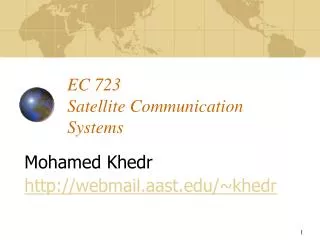
EC 723 Satellite Communication Systems. Mohamed Khedr http://webmail.aast.edu/~khedr. Syllabus. Tentatively. Radio Propagation: Atmospheric Losses. Different types of atmospheric losses can perturb radio wave transmission in satellite systems: Atmospheric absorption;

E N D
EC 723 Satellite Communication Systems Mohamed Khedr http://webmail.aast.edu/~khedr
Syllabus • Tentatively
Radio Propagation: Atmospheric Losses • Different types of atmospheric losses can perturb radio wave transmission in satellite systems: • Atmospheric absorption; • Atmospheric attenuation; • Traveling ionospheric disturbances.
Radio Propagation:Atmospheric Absorption • Energy absorption by atmospheric gases, which varies with the frequency of the radio waves. • Two absorption peaks are observed (for 90º elevation angle): • 22.3 GHz from resonance absorption in water vapour (H2O) • 60 GHz from resonance absorption in oxygen (O2) • For other elevation angles: • [AA] = [AA]90 cosec Source: Satellite Communications, Dennis Roddy, McGraw-Hill
Radio Propagation:Atmospheric Attenuation • Rain is the main cause of atmospheric attenuation (hail, ice and snow have little effect on attenuation because of their low water content). • Total attenuation from rain can be determined by: • A = L [dB] • where [dB/km] is called the specific attenuation, and can be calculated from specific attenuation coefficients in tabular form that can be found in a number of publications; • where L [km] is the effective path length of the signal through the rain; note that this differs from the geometric path length due to fluctuations in the rain density.
Signal Polarisation:Cross-Polarisation Discrimination • Depolarisation can cause interference where orthogonal polarisation is used to provide isolation between signals, as in the case of frequency reuse. • The most widely used measure to quantify the effects of polarisation interference is called Cross-Polarisation Discrimination (XPD): • XPD = 20 log (E11/E12) • To counter depolarising effects circular polarising is sometimes used. • Alternatively, if linear polarisation is to be used, polarisation tracking equipment may be installed at the antenna. Source: Satellite Communications, Dennis Roddy, McGraw-Hill
Illustration of the various propagation loss mechanisms on a typical earth-space path The ionosphere can cause the electric vector of signals passing through it to rotate away from their original polarization direction, hence causing signal depolarization. the sun (a very “hot” microwave and millimeter wave source of incoherent energy), an increased noise contribution results which may cause the C/N to drop below the demodulator threshold. The absorptive effects of the atmospheric constituents cause an increase in sky noise to be observed by the receiver Refractive effects (tropospheric scintillation) cause signal loss. The ionosphere has its principal impact on signals at frequencies well below 10 GHz while the other effects noted in the figure above become increasingly strong as the frequency of the signal goes above 10 GHz
Atmospheric attenuation Attenuation of the signal in % Example: satellite systems at 4-6 GHz 50 40 rain absorption 30 fog absorption e 20 10 atmospheric absorption 5° 10° 20° 30° 40° 50° elevation of the satellite
Signal TransmissionLink-Power Budget Formula • Link-power budget calculations take into account all the gains and losses from the transmitter, through the medium to the receiver in a telecommunication system. Also taken into the account are the attenuation of the transmitted signal due to propagation and the loss or gain due to the antenna. • The decibel equation for the received power is: • [PR] = [EIRP] + [GR] - [LOSSES] Where: • [PR] = received power in dBW • [EIRP] = equivalent isotropic radiated power in dBW • [GR] = receiver antenna gain in dB • [LOSSES] = total link loss in dB • dBW = 10 log10(P/(1 W)), where P is an arbitrary power in watts, is a unit for the measurement of the strength of a signal relative to one watt.
Link Budget parameters • Transmitter power at the antenna • Antenna gain compared to isotropic radiator • EIRP • Free space path loss • System noise temperature • Figure of merit for receiving system • Carrier to thermal noise ratio • Carrier to noise density ratio • Carrier to noise ratio
Signal TransmissionEquivalentIsotropic Radiated Power • An isotropic radiator is one that radiates equally in all directions. • The power amplifier in the transmitter is shown as generating PT watts. • A feeder connects this to the antenna, and the net power reaching the antenna will be PT minus the losses in the feeder cable, i.e. PS. • The power will be further reduced by losses in the antenna such that the power radiated will be PRAD (< PT). (a) Transmitting antenna Source: Satellite Communications, Dennis Roddy, McGraw-Hill
Antenna Gain • We need directive antennas to get power to go in wanted direction. • Define Gain of antenna as increase in power in a given direction compared to isotropic antenna. • P() is variation of power with angle. • G() is gain at the direction . • P0 is total power transmitted. • sphere = 4p solid radians
EIRP - 1 • An isotropic radiator is an antenna which radiates in all directions equally • Antenna gain is relative to this standard • Antennas are fundamentally passive • No additional power is generated • Gain is realized by focusing power • Effective Isotropic Radiated Power (EIRP) is the amount of power the transmitter would have to produce if it was radiating to all directions equally • Note that EIRP may vary as a function of direction because of changes in the antenna gain vs. angle
EIRP Pt Pout Lt HPA EIRP - 2 • The output power of a transmitter HPA is: Pout watts • Some power is lost before the antenna: Pt =Pout/Lt watts reaches the antenna Pt = Power into antenna • The antenna has a gain of: Gt relative to an isotropic radiator • This gives an effective isotropic radiated power of: EIRP = PtGtwatts relative to a 1 watt isotropic radiator
Received Power • We can rewrite the power flux density now considering the transmit antenna gain: • The power available to a receive antenna of area Ar m2 we get:
Effective Aperture • Real antennas have effective flux collecting areas which are LESS than the physical aperture area. • Define Effective Aperture Area Ae: • Where Aphy is actual (physical) aperture area. • Very good: 75% • Typical: 55% • = aperture efficiency • Antennas have (maximum) gain G related to the effective aperture area as follows:
Back to Received Power… • The power available to a receive antenna of effective area Ar = Ae m2 is: Where Ar = receive antenna effective aperture area = Ae Inverting…
Back to Received Power… Friis Transmission Formula • The inverse of the term at the right referred to as “Path Loss”, also known as “Free Space Loss” (Lp): Therefore…
More complete formulation • Demonstrated formula assumes idealized case. • Free Space Loss (Lp) represents spherical spreading only. • Other effects need to be accounted for in the transmission equation: • La = Losses due to attenuation in atmosphere • Lta = Losses associated with transmitting antenna • Lra = Losses associates with receiving antenna • Lpol = Losses due to polarization mismatch • Lother = (any other known loss - as much detail as available) • Lr = additional Losses at receiver (after receiving antenna)
Signal TransmissionLink-Power Budget Formula Variables • Link-Power Budget Formula for the received power [PR]: • [PR] = [EIRP] + [GR] - [LOSSES] • The equivalent isotropic radiated power [EIRP] is: • [EIRP] = [PS] + [G] dBW, where: • [PS] is the transmit power in dBW and [G] is the transmitting antenna gain in dB. • [GR] is the receiver antenna gain in dB. • [LOSSES] = [FSL] + [RFL] + [AML] + [AA] + [PL], where: • [FSL] = free-space spreading loss in dB = PT/PR (in watts) • [RFL] = receiver feeder loss in dB • [AML] = antenna misalignment loss in dB • [AA] = atmospheric absorption loss in dB • [PL] = polarisation mismatch loss in dB • The major source of loss in any ground-satellite link is the free-space spreading loss.
Link Power Budget Tx EIRP Transmission: HPA Power Transmission Losses (cables & connectors) Antenna Gain Antenna Pointing Loss Free Space Loss Atmospheric Loss (gaseous, clouds, rain) Rx Antenna Pointing Loss Reception: Antenna gain Reception Losses (cables & connectors) Noise Temperature Contribution Rx Pr
Translating to dBs • The transmission formula can be written in dB as: • This form of the equation is easily handled as a spreadsheet (additions and subtractions!!) • The calculation of received signal based on transmitted power and all losses and gains involved until the receiver is called “Link Power Budget”, or “Link Budget”. • The received power Pr is commonly referred to as “Carrier Power”, C.
Link Power Budget Now all factors are accounted for as additions and subtractions Tx EIRP • Transmission: • + HPA Power • Transmission Losses • (cables & connectors) • + Antenna Gain • Antenna Pointing Loss • Free Space Loss • Atmospheric Loss (gaseous, clouds, rain) • - Rx Antenna Pointing Loss • Reception: • + Antenna gain • Reception Losses • (cables & connectors) • + Noise Temperature Contribution Rx Pr
Easy Steps to a Good Link Power Budget • First, draw a sketch of the link path • Doesn’t have to be artistic quality • Helps you find the stuff you might forget • Next, think carefully about the system of interest • Include all significant effects in the link power budget • Note and justify which common effects are insignificant here • Roll-up large sections of the link power budget • Ie.: TXd power, TX ant. gain, Path loss, RX ant. gain, RX losses • Show all components for these calculations in the detailed budget • Use the rolled-up results in build a link overview • Comment the link budget • Always, always, always use units on parameters (dBi, W, Hz ...) • Describe any unusual elements (eg. loss caused by H20 on radome)
Why calculate Link Budgets? • System performance tied to operation thresholds. • Operation thresholds Cmin tell the minimum power that should be received at the demodulator in order for communications to work properly. • Operation thresholds depend on: • Modulation scheme being used. • Desired communication quality. • Coding gain. • Additional overheads. • Channel Bandwidth. • Thermal Noise power. We will see more on these items in the next classes.
Closing the Link • We need to calculate the Link Budget in order to verify if we are “closing the link”. Pr >= Cmin Link Closed Pr < Cmin Link not closed • Usually, we obtain the “Link Margin”, which tells how tight we are in closing the link: Margin = Pr – Cmin • Equivalently: Margin > 0 Link Closed Margin < 0 Link not closed
Carrier to Noise Ratios • C/N: carrier/noise power in RX BW (dB) • Allows simple calculation of margin if: • Receiver bandwidth is known • Required C/N is known for desired signal type • C/No: carrier/noise p.s.d. (dbHz) • Allows simple calculation of allowable RX bandwidth if required C/N is known for desired signal type • Critical for calculations involving carrier recovery loop performance calculations
System Figure of Merit • G/Ts: RX antenna gain/system temperature • Also called the System Figure of Merit, G/Ts • Easily describes the sensitivity of a receive system • Must be used with caution: • Some (most) vendors measure G/Ts under ideal conditions only • G/Ts degrades for most systems when rain loss increases • This is caused by the increase in the sky noise component • This is in addition to the loss of received power flux density
System Noise Power - 1 • Performance of system is determined by C/N ratio. • Most systems require C/N > 10 dB. (Remember, in dBs: C - N > 10 dB) • Hence usually: C > N + 10 dB • We need to know the noise temperature of our receiver so that we can calculate N, the noise power (N = Pn). • Tn (noise temperature) is in Kelvins (symbol K):
System Noise Power - 2 • System noise is caused by thermal noise sources • External to RX system • Transmitted noise on link • Scene noise observed by antenna • Internal to RX system • The power available from thermal noise is: where k = Boltzmann’s constant = 1.38x10⁻²³ J/K(-228.6 dBW/HzK), Ts is the effective system noise temperature, andB is the effective system bandwidth
Noise Spectral Density • N = K.T.B N/B = N0 is the noise spectral density (density of noise power per hertz): • N0 = noise spectral density is constant up to 300GHz. • All bodies with Tp >0K radiate microwave energy.
System Noise Temperature 1) System noise power is proportional to system noise temperature 2) Noise from different sources is uncorrelated (AWGN) • Therefore, we can • Add up noise powers from different contributions • Work with noise temperature directly • So: • But, we must: • Calculate the effective noise temperature of each contribution • Reference these noise temperatures to the same location Additive White Gaussian Noise (AWGN)
Typical Receiver (Source: Pratt & Bostian Chapter 4, p115)
Noise Model (Source: Pratt & Bostian Chapter 4, p115) Noise is added and then multiplied by the gain of the device (which is now assumed to be noiseless since the noise was already added prior to the device)
Equivalent Noise Model of Receiver (Source: Pratt & Bostian Chapter 4, p115) Equivalent model: Equivalent noise Ts is added and then multiplied by the equivalent gain of the device, GRFGmGIF (noiseless).
Calculating System Noise Temperature - 1 • Receiver noise comes from several sources. • We need a method which reduces several sources to a single equivalent noise source at the receiver input. • Using model in Fig. 4.5.a gives:
Calculating System Noise Temperature - 2 • Divide by GIFGmGRFkB: • If we replace the model in Fig. 4.5.a by that in Fig. 4.5b
Calculating System Noise Temperature - 3 • Equate Eqns : • Since C is invariably small, N must be minimized. • How can we make N as small as possible?
Reducing Noise Power • Make B as small as possible – just enough bandwidth to accept all of the signal power (C ). • Make TS as small as possible • Lowest TRF • Lowest Tin (How?) • High GRF • If we have a good low noise amplifier (LNA), i.e., low TRF, high GRF, then rest of receiver does not matter that much.
Reducing Noise Power Discussion on Tin • Earth Stations: Antennas looking at space which appears cold and produces little thermal noise power (about 50K). • Satellites: antennas beaming towards earth (about 300 K): • Making the LNA noise temperature much less gives diminishing returns. • Improvements aim reduction of size and weight.
Antenna Noise Temperature • Contributes for Tin • Natural Sources (sky noise): • Cosmic noise (star and inter-stellar matter), decreases with frequency, (negligible above 1GHz). Certain parts of the sky have punctual “hot sources” (hot sky). • Sun (T 12000 f-0.75 K): point earth-station antennas away from it. • Moon (black body radiator): 200 to 300K if pointed directly to it. • Earth (satellite) • Propagation medium (e.g. rain, oxygen, water vapor): noise reduced as elevation angle increases. • Man-made sources: • Vehicles, industrial machinery • Other terrestrial and satellite systems operating at the same frequency of interest.
Antenna Noise Temperature • Useful approximation for Earth Station antenna temperature on clear sky (no rain):
Power Budget Example - 1 4.1.1 Satellite at 40,000 km (range) Transmits 2W Antenna gain Gt = 17 dB (global beam) Calculate: a. Flux density on earth’s surface b. Power received by antenna with effective aperture of 10m2 c. Gain of receiving antenna. d. Received C/N assuming Ts =152 K, and Bw =500 MHz a. Using Eqn. 4.3: (Gt = 17 dB = 50) (Solving in dB…)
Power Budget Example - 1 b. Received Power (Solving in dB…) • c. Gain given Ae = 10 m2 and Frequency = 11GHz ( eqn. 4.7)
Power Budget Example - 1 b. System Noise Temperature
Power Budget Example - 2 Generic DBS-TV: Received Power Transponder output power , 160 W 22.0 dBW Antenna beam on-axis gain 34.3 dB Path loss at 12 GHz, 38,500 km path -205.7 dB Receiving antenna gain, on axis 33.5 dB Edge of beam -3.0 dB Miscellaneous losses -0.8 dB Received power, C -119.7 dBW
Power Budget Example - 2 Noise power Boltzmann’s constant, k -228.6 dBW/K/Hz System noise temperature, clear air, 143 K 21.6 dBK Receiver noise bandwidth, 20MHz 73.0 dBHz Noise power, N -134.0 dBW C/N in clear air 14.3 dB Link margin over 8.6 dB threshold 5.7 dB Link availability throughout US Better than 99.7 %