Download
1 / 78
1k likes | 1.29k Views
V ∞. u o. V ∞. turbulent wake behind body. turbulent wake behind smokestack. y. u o. u ( y ). turbulent jet. CHAPTER 8. CONVECTION IN EXTERNAL TURBULENT FLOW. 8.1 Introduction. Common physical phenomenon, but complex.

E N D
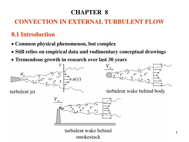
V∞ uo V∞ turbulent wake behind body turbulent wake behind smokestack y uo u(y) turbulent jet CHAPTER 8 CONVECTION IN EXTERNAL TURBULENT FLOW 8.1 Introduction • Common physical phenomenon, but complex Still relies on empirical data and rudimentary conceptual drawings Tremendous growth in research over last 30 years
y u(y,t) u′(y,t) u u(y,t) Instantaneous velocity profile u u(t) Instantaneous velocity fluctuation u velocity profiles t fluctuating component 8.1.1 Examples of Turbulent Flows (i) Mixing Processes (ii) Free Shear Flows (iii) Wall-Bounded Flows • Varying shape of instantaneous velocity profile • Instantaneous velocity fluctuation
u(y) δturb y turbulent δlam laminar u Turbulent velocity profile vs. laminar • Time averaged Turbulent flows can enhanceperformance • Turbulators • Dimpled golf balls
(8.1) • Internal flow: critical flow number is • Flow over semi-infinite flat plate is 8.1.2 The Reynolds Number and the Onset of Turbulence • Osborne Reynolds (1883) first identifies laminar and turbulent regimes • Reynolds number: Why the Reynolds number predicts the onset of turbulence • Reynolds number represents the ratio of inertial to viscous forces • Inertial forces accelerate a fluid particle • Viscous forces slow or damp the motion of the particle • At low velocity, viscous forces dominate • Infinitesimal disturbances damped out • Flow remains laminar
At high enough fluid velocity, inertial forces dominate • Viscous forces cannot prevent a wayward particle from motion • Chaotic flow ensues Turbulence near wall • For wall-bounded flows, turbulence initiates near the wall
(8.2) 8.1.3 Eddies and Vorticity • An eddy is a particle of vorticity, ω, • Eddies typically form in regions of velocity gradient. • Vorticity can be found from Eqn. (8.2) to be A Common View of Eddy Formation • Eddy begins as a disturbance near the wall • Vortexfilament forms • Stretched into horseshoe or hairpin vortex • Lifting phenomenon
8.1.4 Scales of Turbulence • Largest eddies break up due to inertial forces • Smallest eddies dissipate due to viscous forces • Richardson Energy Cascade (1922)
(8.3a) (8.3b) (8.3c) Kolgomorov Microscales (1942) • Attempt to estimate size of smallest eddies • Important impacts: • There is a vast range of eddy sizes, velocities, and time scales • in a turbulent flow. This could make modeling difficult. • The smallest eddies small, but not infinitesimally small. • Viscosity dissipates them into heat before they can become • too small. • Scale of the smallest eddies are determined by the scale of the largest eddies through the Reynolds number. • Generating smaller eddies is how the viscous dissipation is • increased to compensate for the increased production of • turbulence.
The smallest eddies: approximately 8.1.5 Characteristics of Turbulence • Turbulence is comprised of irregular, chaotic, three-dimensional fluid motion, but containing coherent structures. • Turbulence occurs at high Reynolds numbers, where instabilities give way to chaotic motion. • Turbulence is comprised of many scales of eddies, which dissipate energy and momentum through a series of scale ranges. The largest eddies contain the bulk of the kinetic energy, and break up by inertial forces. The smallest eddies contain the bulk of the vorticity, and dissipate by viscosity into heat. • Turbulent flows are not only dissipative, but also dispersive through the advection mechanism. 8.1.6 Analytical Approaches • Considering small eddies, is continuum hypothesis still valid?
Mean free path of air at atmospheric pressure is on the order • of three orders of magnitude smaller • Continuum hypothesis OK • Are numerical simulations possible? • Direct Numerical Simulation (DNS) a widespread topic of • research • However, short time scales and size range of turbulence a • problem • Still have to rely on more traditional analytical techniques Two Common Idealizations • Homogeneous Turbulence: Turbulence, whose microscale motion, on average, does not change from location to location and time to time. • Isotropic Turbulence: Turbulence, whose microscale motion, on average, does not change as the coordinate axes are rotated.
(8.4) (8.5) (8.6) 8.2 Conservation Equations for Turbulent Flow 8.2.1 Reynolds Decomposition • Turbulent flow seems well-behaved on average. • Reynolds Decomposition: Separate velocity, properties into time- averaged and fluctuating components: • Time-averaged component is determined by: • Time average of fluctuating component is zero:
For two variables and (8.7a) (8.7b) (8.7c) (8.7d) (8.7e) (8.7f) (8.7g) (8.7h) (8.7i) (8.7j) Average Identities: 8.2.2 Conservation of Mass
(2.2a) • Assume incompressible, two-dimensional flow. Substituting the Reynolds-decomposed velocities and , (a) (b) (c) • By identities (8.7a) and (8.6): • Expanding, • Time-average the equation: • Then, simplify each term by invoking identity (8.7h):
(8.8) (d) (2.10x) (2.10y) • By identities (8.7a) and (8.6), 8.2.3 Conservation of Momentums • The x and y momentum equations are given by:
(8.10x) (8.10y) • For the x-momentum equation, the terms can be replaced by the following relations, derived from the product rule of derivation: (a) (b) (c) • Simplifying for steady, 2D flow, no body forces: • Substitute (a) into the x-momentum equation (8.10x):
Note that terms marked and in the above can be combined as: (d) (8.11) (8.12x) (8.12y) • Thus, the x-momentum equation reduces to: • Following Reynolds decomposition and averaging, 8.2.4 Conservation of Energy
(2.19b) (8.13) (8.14) • For incompressible flow, negligible heat generation, constant properties, the energy equation is given by • The energy equation reduces to: • Following Reynolds decomposition and time averaging, Eqn. (8.13) becomes: • NOTE TWO NEW TERMS
(8.14) (8.8) (8.12x) (8.12y) 8.2.5 Summary of Governing Equations for Turbulent Flow • Continuity: • x-momentum: • y-momentum: • Energy:
(8.15) (8.16a) (8.16b) (8.16c) 8.3 Analysis of External Turbulent Flow 8.3.1 Turbulent Boundary Layer Equations (i) Turbulent Momentum Boundary Layer Equation • Consider a flat plate in turbulent flow. • Assume boundary layer is thin: • Following the same arguments as for the laminar boundary layer, the following scalar arguments are made:
(8.17) (8.18) (8.19) • It can be shown that the viscous dissipation terms in (8.12x) compare as follows: • Also, the pressure gradient in the y-direction is negligible: • The pressure gradient in the x-direction can be expressed as: Simplifying the Fluctuation Terms: • Fluctuation Terms: • If fluctuation terms are the result of eddies, one could argue that there is no preferred direction to the fluctuations:
(8.20) (8.22) or (8.21) First Fluctuation Term: (a) Second Fluctuation Term: (b) • Since , we conclude that: • Using scale analysis: • The x-momentum equation for the turbulent boundary layer reduces to:
(8.20) (8.26) (8.20) (8.16b) (8.24) (8.25) (ii) Turbulent Energy Equation • Scaling arguments for the thermal boundary is: • Then: • Fluctuation terms: • Assuming there is no preferred direction to the fluctuations:
(8.28) (8.29) (8.31) (8.30) or (8.27) • We can then show that: • The energy equation then reduces to: 8.3.2 Reynolds Stress and Heat Flux • Can write the x-momentum and energy boundary layer equations as:
is called the turbulent shear stress or the Reynolds stress • is called the turbulent heat flux or the Reynolds heat flux • Continuity: (8.8) • Fluctuating term in (8.30) “looks” like a shear stress • Fluctuating term in (8.31) “looks” like a heat flux • Consider a particle “fluctuation” imposed on some average velocity profile 8.3.3 The Closure Problem of Turbulence • Turbulent boundary layer equations:
(8.31) (8.30) (8.31a) (8.31b) (8.31c) (8.31d) (8.31e) (8.31f) (8.31g) (8.32) (8.33) • x-momentum: • Energy: • Boundary conditions: • Also have, outside the boundary layer:
(8.34) (8.35) • is called the momentum eddy diffusivity. • is called the thermal eddy diffusivity. is often referred to as eddy viscosity. is often referred to as eddy conductivity. • Leaves us with three equations (8.8), (8.30) and (8.31), but five unknowns: • This is the closure problem of turbulence. 8.3.4 Eddy Diffusivity • Customary to model the Reynolds stress as • Similarly, we can model the Reynolds heat flux as • We can then write the boundary layer momentum and energy equations as
(8.38) (8.39) (8.40) (8.41) • Simplest model by Boussinesq: constant • does not allow to approach zero at the wall • The terms in brackets represent the apparent shear stress and apparent heat flux, respectively: 8.4 Momentum Transfer in External Turbulent Flow 8.4.1 Modeling Eddy Diffusivity: Prandtl’s Mixing Length Theory
The velocity fluctuation that results can be approximated from a Taylor series as (a) (a) (b) • Prandtl (1925): used analogy to kinetic theory of gases • Define the mixing length l as the distance the particle travels towards the wall as the result of a fluctuation. • Thus,
If we assume, as we have before, that fluctuations have no preferred direction, then , and so • One could argue, then, that the turbulent stress term is of the following scale: (8.42) (8.44) (c) (d) (8.43) • Finally, we can solve Equation (8.34), for the eddy viscosity: • Prandtl proposed the following model for the mixing length, • Leading to Prandtl’s mixing-length model:
First Step: normalize variables: vs. (8.45) (8.46) (8.47) 8.4.2 Universal Turbulent Velocity Profile • One way to solve momentum is to assume a velocity profile, then use approximate methods to solve integral momentum (like in Chap. 5) (i) Large-Scale Velocity Distribution: “Velocity Defect Law” • Doesn’t collapse curves with varying friction Velocity Defect Law • Introduce coefficient of friction: • Second, define a friction velocity as:
(8.48) (8.49) Near the Wall: (8.50) (8.51) • Define velocity defect: • This works, but doesn’t provide enough detail near the wall. (ii) Wall Coordinates • Dimensional analysis suggests the following wall coordinates: (iii) Near-Wall Profile: Couette Flow Assumption • Very close to the wall, scaling analysis suggests:
This result is similar to Couette flow: Couette Flow Assumption • Resulting curve:
First, we need to express (8.51) in terms of the wall coordinates and . Substituting their definitions, it can be shown that: • Very close to the wall, viscous forces dominate, (8.52) (8.53) (8.54) • Integrating, with boundary condition at • What do we do with this? We can use (8.51) to develop an expression for the velocity profile. • And after rearranging and integrating, (iv) Viscous Sublayer • Couette Flow Assumption (8.52) reduces to:
This relation compares well to experimental data from which we call the viscous sublayer. • Further away from the wall, turbulent fluctuations dominate, (8.55) (8.56) (8.57) (v) Fully Turbulent Region: “Law of the Wall” • Couette Flow Assumption (8.52) becomes • Substitute Prandtl’s mixing length, and wall coordinates: • Substitute into Equation (8.55), • Solve for the velocity gradient,
(8.58) (8.59) (8.60) • The constant of integration B can be estimated by noting that the viscous sublayer and the Law of the Wall region appear to intersect at roughly . Using this as a boundary condition, the integration constant is found to be β ≈ 5.0. • Finally, integrate the above to obtain • This is sometimes referred to as the Law of the Wall. • The constant κis called von Karman’s constant, and experimental measurements show that κ ≈ 0.41. • Thus, an approximation for the Law of the Wall region is: (vi) Other Models • van Driest’s continuous law of the wall • van Driest proposed a mixing length model of this form: • van Driest used this equation with (8.42) and (8.51) to obtain:
Transforming (8.61) into wall coordinates, and solving for one can obtain: (8.61) (8.62) (8.63) (8.64) • Spalding’s Law: • Works for flat plate and pipe flow • Reichardt’s Law, applied frequently to pipe flow: (vii) Effect of Pressure Gradient
In the presence of an adverse pressure gradient, the velocity profile beyond deviates from the Law of the Wall model. • The deviation is referred to as a “wake,” and the region is commonly referred to as the wake region, where the velocity profile deviates even from the overlap region. • Law of the Wall-type models developed earlier model flat plate flow reasonably well in the presence of zero pressure gradient. • A favorable pressure gradient is approximately what we encounter in pipe flow, which helps explain why the models developed here apply as well to pipe flow.
(5.5) 8.4.3 Approximate Solution for Momentum Transfer: Momentum Integral Method (i) Prandtl - von Karman Model • Consider a flat, impermeable plate exposed to incompressible, zero-pressure-gradient flow • The integral momentum equation reduces to equation (5.5), • Applies to turbulent flows as well – without modification – if we look at the behavior of the flow on average, and we interpret the flow properties as time-averaged values. Estimate of Velocity Profile • The integral method requires an estimate for the velocity profile in the boundary layer. • Prandtl and von Kármán both used a crude but simple model for the velocity profile using prior knowledge about pipe flow.
(8.65) • To apply the 1/7th law to flat plate, we approximate as the edge of the boundary layer , and approximate as . Then, • Using the Blasius model for the shear at the wall of a circular pipe, Prandtl [18] and von Kármán [16] each showed that the velocity profile in the pipe could be modeled as • This is the well-known 1/7th Law velocity profile, discussed further in Chapter 9. • Why base a velocity profile for flat plate on pipe flow? The velocity data for pipe flow and flat plate flow (at zero or favorable pressure gradient) have essentially the same shape, so the use of this model to describe flow over a flat plate is not unreasonable. Model for Wall Shear • LHS of Integral Momentum is an expression for wall shear; uses assumed velocity profile.
(8.67) • Problem: our assumed profile goes to infinity as y approaches zero. • To avoid this dilemma, Prandtl and von Kármán again looked to pipe flow knowledge • They adapted the Blasius correlation for pipe flow friction factor to find an expression for the wall shear on a flat plate • Recasting the Blasius correlation terms of the wall shear and the tube radius, they obtained • This is used in the LHS of the momentum integral relation. Example 8.2: Integral Solution for Turbulent Boundary Layer Flow over a Flat Plate Consider turbulent flow over a flat plate, depicted in Fig. 8.8. Using the 1/7th law velocity profile (8.65) and the expression for friction factor (8.67), obtain expressions for the boundary layer thickness and friction factor along the plate.
(a) (b) • Dividing the expression by , and collecting terms, (1) Observations. The solution parallels that of Chapter 5 for laminar flow over a flat plate. (2) Problem Definition. Determine expressions for the boundary layer thickness and friction factor as a function of x. (3) Solution Plan. Start with the integral Energy Equation (5.5), substitute the power law velocity profile (8.65) and friction factor (8.67), and solve. (4) Plan Execution. (i) Assumptions. (1) Boundary layer simplifications hold, (2) constant properties, (3) incompressible flow, (4) impermeable flat plate. (ii) Analysis. • Substitute 1/7th power law velocity profile into the Mom. Int. Equation:
(8.68) (c) (8.69) • Can assume that is zero at x = 0, which ignores the initial laminar boundary layer region • After integrating, • Now substituting (a) into the wall shear expression (8.67), • Then, separating variables and integrating, • To complete the solution, a boundary condition is needed. • However crude the assumption, we find that the results of this analysis compare well to experimental data.
With the boundary condition established, the integration constant C equals zero. Then solving (8.69) for , or (8.70) (d) (e) (8.71) • Finally, solve for the friction factor. Substituting (8.70) into (8.67), Which reduces to (5) Checking. Equations (8.70) and (8.71) are both dimensionless, as expected.
(6) Comments. Note that, according to this model, the turbulent boundary layer δ/x varies as , as does the friction factor . This is contrast to laminar flow, in which δ/x and vary as . • First, substituting the definitions of and , as well as , into the Law of the Wall expression (8.59), • In theory, any y value within the wall law layer would satisfy this expression, but a useful value to choose is the edge of the boundary layer, where . Then, the above can be expressed as (ii) Newer Models • One limitation of the Prandtl-von Kármán model is that the approximation for the wall shear, Eqn. (8.66), is based on limited experimental data, and considered to be of limited applicability even for pipe flow. White’s Model • White [14] uses the Law of the Wall velocity profile (8.59) to model the wall shear.
Still a difficult relation to use, but a simpler curve fit over a range of values from gives (8.72) and (8.75) (8.73) (8.74) • We can now use this expression to estimate the wall shear in the integral method. • For the velocity profile, the 1/7th power law is still used. • It can be shown that the solution to the momentum integral equation in this case becomes • Equations (8.74) and (8.75) replace the less accurate Prandtl-von Kármán correlations, and White recommends these expressions for general use.
(8.76) (8.76) Kestin and Persen’s Model • Perhaps a more accurate correlation would result if we use one of the more advanced velocity profiles to estimate the wall shear, as well as to replace the crude 1/7th power law profile. • Kestin and Persen used Spalding’s law of the wall for the velocity profile and shear stress. • The resulting model is extremely accurate, but cumbersome. White [20] modified the result to obtain the simpler relation • White reports that this expression is accurate to within 1% of Kestin and Persen’s model. (iii) Total Drag • The total drag is found by integrating the wall shear along the entire plate. Assuming the presence of an initial laminar flow region,
Dividing by , the drag coefficient is: • Assume (8.78) (8.79) • Substituting Eqn. (4.48) for laminar flow and using White’s model (8.75) for turbulent flow, we obtain with some manipulation, 8.4.4 Effect of Surface Roughness on Friction Factor • The interaction between the already complex turbulent flow and the complex, random geometric features of a rough wall is the subject of advanced study and numerical modeling. • However, with crude modeling and some experimental study we can gain at least some physical insight. • Define k as the average height of roughness elements on the surface. In wall coordinates:
Experiments show that for small values of (less than approximately 5), the velocity profile and friction factor are unaffected by roughness • For or so, however, the roughness extends beyond the viscous sublayer, and the viscous sublayer begins to disappear, likely due to the enhanced mixing in the roughness provided. • Beyond viscous effects are virtually eliminated, and the flow is referred to as fully rough. Beyond this value of roughness, the shape of the velocity profile changes very little. Consequently, we might expect that once the surface is fully rough, increasing the roughness would not change the friction factor.
(2.52) (8.81) • Turbulence introduces two new variables into the analysis: the momentum and thermal eddy diffusivities, . 8.5 Energy Transfer in External Turbulent Flow • Not surprisingly, energy transfer is also greatly complicated under turbulent flow. • We found in Chapter 2 that the heat transfer for flow over a geometrically similar body like a flat plate (neglecting both buoyancy and viscous dissipation) could be correlated through dimensionless analysis by • One way to deal with these new terms is to introduce a new dimensionless parameter: Turbulent Prandtl Number Approaches to Analyzing Turbulent Heat Transfer • Find a mathematical analogy between heat and mass transfer • Develop a universal temperature profile, similar to how we developed a universal velocity profile.