Download
1 / 24
240 likes | 274 Views
S-052 Fall 2006: Other Questions. DATA INTIMATE; INFILE 'C:Documents and SettingsmillerraDesktopINTIMATE.txt'; INPUT M_SELDIS M_TRUS M_CARE M_VULN M_PHYS M_CRES B_SELDIS B_TRUS B_CARE B_VULN B_PHYS B_CRES; LABEL M_SELDIS = 'self-disclosure with mother'

E N D
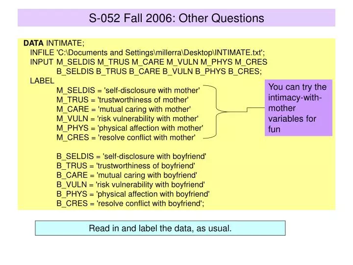
S-052 Fall 2006: Other Questions DATA INTIMATE; INFILE 'C:\Documents and Settings\millerra\Desktop\INTIMATE.txt'; INPUT M_SELDIS M_TRUS M_CARE M_VULN M_PHYS M_CRES B_SELDIS B_TRUS B_CARE B_VULN B_PHYS B_CRES; LABEL M_SELDIS = 'self-disclosure with mother' M_TRUS = 'trustworthiness of mother' M_CARE = 'mutual caring with mother' M_VULN = 'risk vulnerability with mother' M_PHYS = 'physical affection with mother' M_CRES = 'resolve conflict with mother' B_SELDIS = 'self-disclosure with boyfriend' B_TRUS = 'trustworthiness of boyfriend' B_CARE = 'mutual caring with boyfriend' B_VULN = 'risk vulnerability with boyfriend' B_PHYS = 'physical affection with boyfriend' B_CRES = 'resolve conflict with boyfriend'; You can try the intimacy-with-mother variables for fun Read in and label the data, as usual.
S-052 Fall 2006: Other Questions PROCPRINT DATA=INTIMATE(obs=20); VAR M_SELDIS M_TRUS M_CARE M_VULN M_PHYS M_CRES; PROCPRINT DATA=INTIMATE (obs=20); VAR B_SELDIS B_TRUS B_CARE B_VULN B_PHYS B_CRES; PROCCORR ALPHA NOMISS DATA=INTIMATE; VAR B_SELDIS B_TRUS B_CARE B_VULN B_PHYS B_CRES; Check that the data read was successful Run a classical item analysis
S-052 Fall 2006: DAM #7 Walkthrough • 3.a. Estimate Cronbach’s alpha for a standardized composite of the six indicators of intimacy. On the output alongside the estimated reliability, write one sentence stating and interpreting the estimate and providing a conclusion about the internal consistency of the set of six indicators. Nearly three-quarters (73%) of the variance in the standardized composite of the six indicators is variance in true scores. The standardized composite is a moderately reliable measure of construct. Raw vs. Standardized: What does the similarity in alpha tell us?
S-052 Fall 2006: DAM #7 Walkthrough • 3.b Conduct a “deleted-item” reliability-based item analysis of the six indicators and, on the output near the item-analysis, write one sentence summarizing your conclusion. The reliability of a standardized composite improves when either B_CARE or B_PHYS is omitted.
S-052 Fall 2006: Other Questions PROCPRINCOMP DATA=INTIMATE OUT=INTIMATE PREFIX=I_; VAR B_SELDIS B_TRUS B_CARE B_VULN B_PHYS B_CRES; PROCUNIVARIATE DATA=INTIMATE; VAR I_1 I_2; PROCSORT DATA=INTIMATE OUT=SORT1; BY I_1 B_SELDIS B_TRUS B_CARE B_VULN B_PHYS B_CRES; PROCPRINT DATA=SORT1; VAR I_1 B_SELDIS B_TRUS B_CARE B_VULN B_PHYS B_CRES; PROCSORT DATA=INTIMATE OUT=SORT2; BY I_2 B_SELDIS B_TRUS B_CARE B_VULN B_PHYS B_CRES; PROCPRINT DATA=SORT2; VAR I_2 B_SELDIS B_TRUS B_CARE B_VULN B_PHYS B_CRES; Conduct modern PCA Inspect individuals with high values on the two principal components of note.
S-052 Fall 2006: DAM #7 Walkthrough • 3.d. Based on the PCA output, construct a scree plot showing the eigenvalues as a function of component number and, on the plot, write one sentence specifying what you believe is the dimensionality of the six indicators of intimacy with the boyfriend and explaining why. Scree The Rule of One and the scree plot offer support for two underlying dimensions of intimacy with boyfriend.
S-052 Fall 2006: DAM #7 Walkthrough • 3.e. Using the strategies demonstrated in class, write an interpretive sentence describing how the dimensions can be interpreted substantively. Girls with high values on I_1 (the first principal component) have uniformly high values across the six indicators. We strive to ascribe a name to this composite. Boldfaced indicators dominate I_1
S-052 Fall 2006: DAM #7 Walkthrough • 3.e. Using the strategies demonstrated in class, write an interpretive sentence describing how the dimensions can be interpreted substantively. Girls with high values on I_2 (the second principal component) have high values on B_CARE and B_PHYS but moderate values on other indicators. We strive to ascribe a name to this composite. Boldfaced indicators dominate I_2
S-052 Fall 2006: Other Questions PROCVARCLUS HIERARCHY DATA=INTIMATE OUTTREE=TREEDAT; VAR B_SELDIS B_TRUS B_CARE B_VULN B_PHYS B_CRES; PROCTREE DATA=TREEDAT; HEIGHT _PROPOR_; PROCPRINCOMP DATA=INTIMATE OUT=INTIMATE PREFIX=G1; VAR B_CARE B_PHYS; PROCPRINCOMP DATA=INTIMATE OUT=INTIMATE PREFIX=G2; VAR B_SELDIS B_TRUS B_VULN B_CRES; Run an exploratory cluster analysis of the 6 predictors Obtain a tree-plot Create the slightly correlated but somewhat cleaner measures of two dimensions of girls’ intimacy with boyfriend
S-052 Fall 2006: DAM #7 Walkthrough 4. Use PROC VARCLUS to cluster the six indicators of intimacy with the boyfriend, obtaining a suitable tree diagram. The first principal components in the 2 clusters offer 63.7% of the variance contained in the standardized indicators. Can we find out about the reliability of these new composites?
P CA T S V CR S-052 Fall 2006: DAM #7 Walkthrough 4. Use PROC VARCLUS to cluster the six indicators of intimacy with the boyfriend, obtaining a suitable tree diagram. We confirm the clusters by graphing the loadings from I_1 and I_2. 0.6 0.6 I_1 I_2
S-052 Fall 2006: Other Questions Both exploratory techniques can tell you about dimensionality within a set of indicators of supposedly the same construct. For a small number of indicators, the PCA has the advantage of giving you a choice between mutually orthogonal dimensions or, with some manipulation, some slightly correlated but perhaps more sensible dimensions. Cluster Analysis only surfaces the latter. For n indicators, there’s n units of standardized variance, and it could turn out that more than three eigenvalues are plenty greater than one. You won’t be able to visualize the slightly correlated dimensions, but Cluster Analysis will take you right to them. PCA will tell you how many clusters to settle on. PCA vs. Cluster Analysis
S-052 Fall 2006: Other Questions How is it that the principal components with loadings on all the indicators in a PCA can be totally uncorrelated while the cluster analysis results, which clump indicators into separate groups, are correlated? PCA finds as many eigenvectors as there are indicators. It gives a purely mathematical solution, one property of which is zero inter-correlation between pairs of principal components. Think of the small loadings on some indicators in some of the principal components as mathematical fine-tuning. If you ignore this fine tuning, composites formed from with the groups of indicators can be somewhat inter-correlated.
S-052 Fall 2006: Other Questions What are log-odd, odds, and odds-ratios from a conceptual perspective? Fitted odds-ratios are very abstract, but they have the nicest relationship to parameter estimates of all options available. Namely, if the log-odds that Y=1 is given by A+BX, then EXP(B) is the odds that Y=1 when X=N+1 divided by the odds that Y=1 when X=N.
S-052 Fall 2006: Other Questions What’s the linearity in the log-odds assumption again? Say log-odds that Y=1 is given by A+BX. Clearly, this means that the log-odds increases by B units when X increases by 1 unit. Unless this is reasonably true in the sample, then fitting the logistic model may produce weird results. We generally have to do clever things to check this: find average values (probabilities) of Y in different X-bins, form odds from the averages, compute log-odds of these, and plot these against the bins. A one unit increase in X certainly does not translate to a fixed increase in the probability of Y=1 (the outcome in the actual model). Thus, the linear assumption is hidden when we look at the logistic model.
S-052 Fall 2006: Other Questions • Purposes • Model building • Compare nested models to test groups of predictors • Contain Type-I error • Test post-hoc hypotheses about the population • Settings • OLS • Scaled difference in SSModel gives an F-statistic • Multilevel and Logistic (iterative fitting by Max. Likelihood) • Scaled difference in -2LL gives a Chi-square statistic for nested models • Use the statistic the computer offers for other GLH (post-hoc or non-nested comparisons) GLH Testing Overview
S-052 Fall 2006: Other Questions Why does SAS give us a “Wald Chi-Square” statistic for the post-hoc GLH test result? Unless models fit by ML are nested, we don’t know that the difference in -2LL has a Chi-square distribution. Thus, for post-hoc tests (where it’s often not even clear that you’re comparing two models), we often have to live with what we do know: Wald statistics, asymptotically, have a Chi-square distribution. For large samples, the decisions supported by either test are rarely different (Afifi). Thus, Wald statistics would be safe to use there for any testing purpose. In small samples, the tests may disagree. But only the Wald statistic is available when the GLH hypothesis does not speak to nested models. This kind of limitation happens all the time in real work. For example, one always violates assumptions at least a little. The question is how to argue that you’ve done everything within reason to ensure your results mean what you think they mean. One main function of journal reviewers is to request additional work along these lines.
S-052 Fall 2006: Other Questions In DAM 6, you performed a post-hoc GLH test. The null could have been written like this: You found a test statistic, Wald Chi-squared = 18.9, df=1, p<.0001. You reject the null, and you say, on average, in the population, adolescents in their 13th year have a different (lower) risk of arrest than adolescents in their 15th year. On the other hand, if you test this hypothesis, You would not reject the null. Although you don’t accept the null, you would wind up saying something that sounds a lot like it. Decisions about hypothesis tests: correct vs. natural language
S-052 Fall 2006: Other Questions When evaluating linear models, when is it appropriate to look at the studentized residuals rather than raw residuals? Studentized residuals are a more complicated cousin of simply standardized residuals. Either kind plotted against predicted outcome can provide mild evidence as to normality (95% within 2 standard units of zero). We like raw residuals plotted against the predictors and the predicted outcome to assess linearity. They amplify non-linearity and the vertical units mean something. The actual assumption of normality concerns the error. The raw residuals are estimates of these errors based on data. Thus, they should be used to test normality in the more formal way (Wilk-Shapiro Test, Normal Prob. Plot). The press (deleted) residuals are useful for identifying individuals with extreme values on the outcome variable. Note: you can often make the right decisions looking at the wrong kind of residuals. Looking at all is more than many researchers do. But it’s best to be a bit careful.
S-052 Fall 2006: Other Questions What do you use to determine that there’s a “strong” vs. “weak” relationship in comparing the effect of two predictors on an outcome? • Say we’ve fit this model • We also know the sample standard deviations for Y, A, and B are 15.7, 0.3, and 1.5 respectively. Obviously, • Δ A=1 ~ ΔY=12.4 • Δ B=1~ ΔY= 0.5 • Less obviously • Δ A=0.3 ~ ΔY=12.4*0.3 or 23.7% of 15.7 • Δ B=1.5 ~ ΔY=0.5*1.5 or 4.8% of 15.7 • Thus, although the coefficient on A is 25 times the coefficient on B, the effect of a 1 SD increase in A, as a fraction of an SD of Y, is only 5 times the effect of a 1SD increase in B, as a fraction of an SD of Y.
S-052 Fall 2006: Other Questions How much testing and assumption-checking should be done at each stage of model building? You cannot test and check everything. Stop at sensible places and dig in. For example, build a baseline control models testing groups of predictors on the way. Then check residuals against predicted values and predictors. Transform a few predictors, if indicated. Now add question predictors, test and check. Now add interactions with question predictors, test and check. If your data is structured such that OLS residuals are not independent, adjust your methods first so you can believe your test results. If your pretty thorough in getting to your final model, you can probably skip a lot of the checking in sensitivity analyses. Keep a diary of the data analyses you did last summer (especially with notes and comments in your data-analytic software). Share highlights of your diary in your paper!
S-052 Fall 2006: Other Questions What about missing values? • There is very often a systematic relationship between individuals with missing values. If this relationship is unobserved, it’s a big problem. Imputing values to replace the missing ones cannot respect the unobserved relationship. Thus, all imputation is suspect. That said, there are some responsible ways to proceed. • Impute values in a way that other scholars have done (substance, theory, method). • Create dummy variables denoting groups of individuals with imputed values. • Conduct sensitivity analyses and present or mention these in findings, appendices or footnotes. • If your findings depend on imputed values, publication may not be in the cards. • However, your qualifications as a scholar are on full display—you graduate.
S-052 Fall 2006: Other Questions Yes, but you would not be in the program but for your passion for substance and theory. Thus, embrace and learn the methods crucial to your area. Work with people of like minds in this respect, especially ones with much fuller minds. Try to keep your initial work simple. In real life you sometime stand in front of the data without knowing how to start.
S-052 Fall 2006: Other Questions As we move forward into our own data analysis, what are the resources at HGSE for getting help? When and under what circumstances is it OK to ask for professor help? This might also include a short overview of which classes are matched to which types of methodologies and data. Any cautionary tales about the type of data we can reasonably expect to collect as doctoral students? The type of analysis we might do? You mentioned frequently during the class that some types of data are hard to collect and/or hard to believe.