Download
1 / 65
650 likes | 666 Views
Learn about linear systems, their properties, and how to analyze and manipulate them using convolution. Explore examples and practice with MATLAB.

E N D
Review: Linear Systems • We define a system as a unit that converts an input function into an output function. Independent variable System operator
Linear Systems • Let where fi(x) is an arbitrary input in the class of all inputs {f(x)}, and gi(x) is the corresponding output. • If Then the system H is called a linear system. • A linear system has the properties of additivity and homogeneity.
Linear Systems • The system H is called shift invariant if for allfi(x) {f(x)} and for allx0. • This means that offsetting the independent variable of the input by x0 causes the same offset in the independent variable of the output. Hence, the input-output relationship remains the same.
Linear Systems • The operator H is said to be causal, and hence the system described by H is a causal system, if there is no output before there is an input. In other words, • A linear system H is said to be stable if its response to any bounded input is bounded. That is, if where K and c are constants.
Linear Systems • A unit impulse function, denoted (a), is defined by the expression (x-a) (a) a x
Linear Systems • A unit impulse function, denoted (a), is defined by the expression Then
Linear Systems • The term is called the impulse response of H. • From the previous slide • It states that, if the response of H to a unit impulse [i.e., h(x, )], is known, then response to any input f can be computed using the preceding integral. In other words, the response of a linear system is characterized completely by its impulse response.
Linear Systems • If H is a shift-invariant system, then and the integral becomes • This expression is called the convolution integral. It states that the response of a linear, fixed-parameter system is completely characterized by the convolution of the input with the system impulse response.
Linear Systems • Convolution of two functions is defined as • In the discrete case
Linear Systems • In the 2D discrete case is a linear filter.
1 1 1 -1 2 1 -1 -1 1 Convolution Example h f Rotate From C. Rasmussen, U. of Delaware
2 2 2 3 5 2 1 3 3 2 2 1 2 1 3 2 2 1 1 1 2 2 2 3 Convolution Example Step 1 -1 2 1 2 1 3 3 -1 -1 1 2 2 1 2 h 1 3 2 2 1 1 1 -1 4 2 -1 -2 1 f*h f From C. Rasmussen, U. of Delaware
2 2 2 3 2 1 3 3 2 2 1 2 1 3 2 2 1 1 1 2 2 2 3 Convolution Example Step 2 -1 2 1 2 1 3 3 -1 -1 1 2 2 1 2 h 1 3 2 2 1 1 1 5 4 -2 4 2 -2 -1 3 f*h f From C. Rasmussen, U. of Delaware
2 2 2 3 5 4 4 2 1 3 3 2 2 1 2 1 3 2 2 1 1 1 2 2 2 3 Convolution Example Step 3 -1 2 1 2 1 3 3 -1 -1 1 2 2 1 2 h 1 3 2 2 1 1 1 -2 4 3 -1 -3 3 f*h f From C. Rasmussen, U. of Delaware
2 2 2 3 5 4 4 -2 2 1 3 3 2 2 1 2 1 3 2 2 1 1 1 2 2 2 3 Convolution Example Step 4 -1 2 1 2 1 3 3 -1 -1 1 2 2 1 2 h 1 3 2 2 1 1 1 -2 6 1 -3 -3 1 f*h f From C. Rasmussen, U. of Delaware
2 2 2 3 5 4 4 -2 2 1 3 3 9 2 2 1 2 1 3 2 2 1 1 1 2 2 2 3 Convolution Example Step 5 -1 2 1 2 1 3 3 -1 -1 1 2 2 1 2 h 1 3 2 2 1 2 2 -1 4 1 -1 -2 2 f*h f From C. Rasmussen, U. of Delaware
2 2 2 3 5 4 4 -2 2 1 3 3 9 6 2 2 1 2 1 3 2 2 1 1 1 2 2 2 3 Convolution Example Step 6 -1 2 1 2 1 3 3 -1 -1 1 2 2 1 2 h 1 3 2 2 2 2 2 -2 2 3 -2 -2 1 f*h f From C. Rasmussen, U. of Delaware
Convolution Example and so on… From C. Rasmussen, U. of Delaware
Example = *
Example = *
MATLAB • Review your matrix-vector knowledge • Matlab help files are helpful to learn it • Exercise: f = [1 2; 3 4] g = [1; 1] g = [1 1] g’ z = f * g’ n=0:10 plot(sin(n)); plot(n,sin(n)); title(‘Sinusoid’); xlabel(‘n’); ylabel(‘Sin(n)’); n=0:0.1:10 plot(n,sin(n)); grid; figure; subplot(2,1,1); plot(n,sin(n)); subplot(2,1,2); plot(n,cos(n));
MATLAB • Some more built-ins a = zeros(3,2) b = ones(2,4) c = rand(3,3) %Uniform distribution help rand help randn %Normal distribution d1 = inv(c) d2 = inv(rand(3,3)) d3 = d1+d2 d4 = d1-d2 d5 = d1*d2 d6 = d1.*d3 e = d6(:)
MATLAB • Image processing in Matlab x=imread(‘cameraman.tif’); figure; imshow(x); [h,w]=size(x); y=x(0:h/2,0:w/2); imwrite(y,’man.tif’); % To look for a keyword lookfor resize
MATLAB • M-file • Save the following as myresize1.m function [y]=myresize1(x) % This function downsamples an image by two [h,w]=size(x); for i=1:h/2, for j=1:w/2, y(i,j) = x(2*i,2*j); end end • Compare with myresize2.m function [y]=myresize2(x) % This function downsamples an image by two [h,w]=size(x); for i=0:h/2-1, for j=0:w/2-1, y(i+1,j+1) = x(2*i+1,2*j+1); end end • Compare with myresize3.m function [y]=myresize3(x) % This function downsamples an image by two y = x(1:2:end,1:2:end); • We can add inputs/outputs function [y,height,width]=myresize4(x,factor) % Inputs: % x is the input image % factor is the downsampling factor % Outputs: % y is the output image % height and width are the size of the output image y = x(1:factor:end,1:factor:end); [height,width] = size(y);
Try MATLAB f=imread(‘saturn.tif’); figure; imshow(f); [height,width]=size(f); f2=f(1:height/2,1:width/2); figure; imshow(f2); [height2,width2=size(f2); f3=double(f2)+30*rand(height2,width2); figure;imshow(uint8(f3)); h=[1 1 1 1; 1 1 1 1; 1 1 1 1; 1 1 1 1]/16; g=conv2(f3,h); figure;imshow(uint8(g));
EE 7730 Edge Detection
Detection of Discontinuities • Matched Filter Example >> a=[0 0 0 0 1 2 3 0 0 0 0 2 2 2 0 0 0 0 1 2 -2 -1 0 0 0 0]; >> figure; plot(a); >> h1 = [-1 -2 2 1]/10; >> b1 = conv(a,h1); figure; plot(b1);
Detection of Discontinuities • Point Detection Example: • Apply a high-pass filter. • A point is detected if the response is larger than a positive threshold. • The idea is that the gray level of an isolated point will be quite different from the gray level of its neighbors. Threshold
Detection of Discontinuities • Point Detection Detected point
Detection of Discontinuities • Line Detection Example:
Detection of Discontinuities • Line Detection Example:
Detection of Discontinuities • Edge Detection: • An edge is the boundary between two regions with relatively distinct gray levels. • Edge detection is by far the most common approach for detecting meaningful discontinuities in gray level. The reason is that isolated points and thin lines are not frequent occurrences in most practical applications. • The idea underlying most edge detection techniques is the computation of a local derivative operator.
Origin of Edges • Edges are caused by a variety of factors surface normal discontinuity depth discontinuity surface color discontinuity illumination discontinuity
Image gradient • The gradient of an image: • The gradient points in the direction of most rapid change in intensity • The gradient direction is given by: • The edge strength is given by the gradient magnitude
Edge Detection • The gradient vector of an image f(x,y) at location (x,y) is the vector • The magnitude and direction of the gradient vector are • is also used in edge detection in addition to the magnitude of the gradient vector.
The discrete gradient • How can we differentiate a digital image f[x,y]? • Option 1: reconstruct a continuous image, then take gradient • Option 2: take discrete derivative (finite difference)
Effects of noise • Consider a single row or column of the image • Plotting intensity as a function of position gives a signal
Look for peaks in Solution: smooth first
Derivative theorem of convolution • This saves us one operation:
Laplacian of Gaussian • Consider Laplacian of Gaussian operator Zero-crossings of bottom graph
2D edge detection filters • is the Laplacian operator: Laplacian of Gaussian Gaussian derivative of Gaussian
The Canny edge detector • original image (Lena)
The Canny edge detector • norm of the gradient
The Canny edge detector • thresholding
The Canny edge detector • thinning • (non-maximum suppression)
Non-maximum suppression • Check if pixel is local maximum along gradient direction • requires checking interpolated pixels p and r
Predicting the next edge point Assume the marked point is an edge point. Then we construct the tangent to the edge curve (which is normal to the gradient at that point) and use this to predict the next points (here either r or s).
Hysteresis • The threshold used to find starting point may be large in following the edge. • This leads to broken edge curves. • The trick is to use two thresholds: A large one when starting an edge chain, a small one while following it.