Download

1 / 26
260 likes | 268 Views
Viewing your results from the PAW Pipeline. Proteomics Shared Resource OHSU. Overview. This document is designed to walk you through the basic results files from the PAW Pipeline.

E N D
Viewing your results from the PAW Pipeline Proteomics Shared Resource OHSU
Overview • This document is designed to walk you through the basic results files from the PAW Pipeline. • It is easiest to view the results in excel. However we also provide tab-delinated text files which should be useable with other spreadsheet programs. However please let us know if you’re having problems opening your results. • The PAW Pipeline was written by Phil Wilmarth of OHSU, you can find the publication here: http://www.springerlink.com/content/9x5rk68628506216/fulltext.pdf • In short the PAW Pipeline is an improvement over the traditional peptide and protein prophet algorithms, and is comparable in sensitivity to some of the best software on the market. • PAW is best suited to the analysis of large datasets, and can be used to more stringently filter data for PTM analysis. It is frequently used by PSR as it often has usually has more sensitivity then Scaffold or Proteome Discoverer.
Your Results Files • There will usually be 4 different results files that come in an e-mail. • One is this powerpoint, which may be in a .pdf format. • There are also 2 text files which contain raw output from the PAW Pipeline. • The bulk of the relevant results will be contained in the excel file, which we’ll go over first.
Excel File Your initial results file will look something like the picture on the right. This can be a little overwhelming at first, as there is a lot of information. So lets break down what each of these columns are.
Column A • Column A orders the proteins by an arbitrary protein number. • It also groups proteins whose identified peptides were indistinguishable by the same integer • For example, proteins 28, 28 & 28.01 have indistinguishable sequence coverage, and so are grouped together.
Column B The total number of visible protein entries is recorded here. • Column B contains a counter row. • The 1’s in each visible row are totaled in cell B4 at the top. • This allows you to sort and filter the data in different ways, and have a count of the number of proteins passing the current set of filters.
Columns C & D • Column C lists the accession number for the identified protein • These come from the swissprot, ensembl, or ncbi database accessed used for the database search. • Column D contains links, that when clicked, should lead you to the protein entry online. • Accession #’s containing ‘CONT_’ are common contaminates added to the database by PSR. • ‘REV_’ are reversed protein entries used by PSR to estimate the false positive rate. • ‘EXTRA_’ indicates protein sequences given to PSR by a client. These entries are an internal control used in the analysis and can generally be ignored
Column E Using these small arrows lets you filter your data by choosing to include or exclude different terms or values from the column. • Column E is a row used to filter out entries we don’t want to appear in the results list. • Typicially the filter is set to hide all contaminant, redundant, and reversed protein entries • This column may also be used at times to filter the data in other ways.
Columns F, G & H • Column F lists the % of the protein sequence in the database found in MS/MS spectra. • The number is combined across all the samples, so sample to sample difference in coverage isn’t visible here. • Column G lists the length of the protein sequence in # of amino acids • Column H gives the calculated molecular weight of the protein in daltons.
Column I • Column I contains a description of the protein. • This is the description included in the .fasta database used in the Sequest search. • descriptions of ‘EXTRA_’ proteins are often added manually by the PSR Staff, who make an attempt to keep the description in-line with information from the client
Columns J, K & L • Column J lists the total number of MS/MS spectra matching to the protein (summed over all samples). • Column K lists the total number of MS/MS spectra matching to ONLY that protein. • Column L displays the fraction of MS/MS spectra that are unique to the protein. This is essentially Column K/Column J. • Column L is important when assessing relative quantitation, and is highlighted yellow when the fewer than 75% of the MS/MS spectra match uniquely to the protein. • When Column L is yellow it can be more difficult to assess quantitative differences between samples for the protein, as it shares a large percentage of sequence with other proteins that may not necessarily share the same abundance differences.
Sample Results Columns • The next several columns will list the total, unique and correct spectral counts across all of the submitted samples. • There will be a total, unique and correct column for each sample, so the total number of columns will vary. • The total column will be colored green for samples where the protein was found. • The intensity of the green background changes with the number of spectra. Divisions are at 1, 5, 10, 30, 100, and 300.
‘Total’ Columns • The ‘total’ column lists the total number of MS/MS spectra matching the protein in the sample listed on the in the 2nd cell of the column. • These columns will often be renamed to have the sample name in the header row.
‘Unique’ Columns • The unique columns list the number of MS/MS spectra that match ONLY to the protein in that particular sample • In cases where there are counts in the ‘total’ column, but not in the ‘unique’ column, there is no direct evidence for the protein in that sample. • Sample with a low number in the unique column, compared to the ‘total’ column, are difficult to compare between samples. This protein has no unique evidence for it in the 2nd sample, meaning it is not necessarily present in that sample.
‘Corrected’ Columns • The corrected columns adjust the spectral count numbers from the total column, and make the values more accurate. • In short, the Corrected total is the Unique total plus a fraction of the “shared” peptides (determined by the relative unique counts of the respective proteins). The total may also be scaled by a normalization factor. • An additional correction is added to give proteins that are not present a non-zero number, as this is necessary in some optional follow-up analyses. • The corrected numbers can generally be ignored in most cases, such as in a Co-IP experiment. Most quantitative work at PSR is now done through TMT isotopic tags, as these are more reliable indicators.
When the corrected numbers are inaccurate • There are a couple of conditions that must be true for the corrected numbers to be accurate. • There should be the same amount of total protein in each sample, within reason, in the initial experiment. • When column L is highlighted yellow, the corrected number might be inaccurate. Estimates of protein abundance should be checked by taking into account changes to the protein, plus all of the proteins listed in the final column of the spreadsheet as a group. • If the normalization numbers are greater than 1.5 or less than 0.67, the correction may be too great to use the corrected numbers. Check housekeeping proteins for consistency. This final column lists any other proteins with overlapping sequence that have been identified in the experiment.
The Two Text Files • The #_protein_summary.txt file is the unedited/unformatted version of the excel spreadsheet. • This file can be used as a backup if you lose or unintentionally edit the excel document in a way you can’t undo. • You can open the file directly into excel and save it as an .xls file. • From that point it should behave like any other excel document • The #_peptide_summary.txt file contains a list of all the peptide sequences identified in the analysis. • It will also mark the location of modification sites, if they were included in the initial analysis. • A formatted version of this text file will be included as an excel document if you requested PTM analysis. • This file can be opened in excel and examined. • More detailed peptide files are also available to satisfy publication requirements of some journals.
Examining the peptide text file • To open the file in excel you’ll want to right click on the file • Then select ‘Open With’ -> Excel • Opening the document will display something similar to what is on the next page
Peptide Text File • The opened peptide text file should look something like what you see on the right. • These files can be quite large, this particular example contains about 900 proteins and about 8,000 lines. • Because of the file size some formatting will likely be necessary to view the results.
Basic Formatting First step is to freeze the panes with the 2nd row selected. This way the header rows are visible when you scroll Next choose to auto-filter with the top row selected. This will allow you to filter individual columns Adding border lines can also aid readability
Formatting Continued • Adjust the width of the columns as necessary. • Finally the addition of conditional formatting in the sample columns can be very helpful.
Conditional Formatting A simple filter would be anything equal to or greater than one. This will highlight samples a peptide is present in You can also set additional filters at different numbers of counts to see abundance differences
Save and View Results Finally save the file in an excel format to preserve the formatting changes. At this point you should be able to select your proteins of interest from the dropdown menu in column B and inspect peptides belonging to each protein. The column A group numbers are the same as in the protein summary File and can also be used to find the proteins of interest. Modifications are marked in the sequence with symbols such as &, # or *. If you are expecting modified peptides in your sample, a key to which modifications are which symbol should be included in the initial e-mail.
Grouped Summary Files Grouped summary files are similar to the normal summary files, and are used when a strict quantitative experiment is being done using spectral counts or ms2 intensities. There are two major differences between this and the normal results files. First there is the _family designation. This denotes instances where multiple very similar proteins were combined into a single entry to aid in quantitative assessment. These entries have too many shared peptides to be considered individually.
Grouped Summary Files Also there are now 3 columns for different degrees of sequence overlap in identified proteins. Identical: accessions of other proteins that are indistinguishable based on evidence seen in the samples. Similar: Accessions of similar proteins that were grouped into families Other Loci: Accessions which share smaller amount of sequence, and therefore were not grouped together.
That’s all! Thanks for reading! • If you have questions about viewing your results please contact us: • (503) 418-1280 • Ashok Reddy: reddyas@ohsu.edu • Jennifer Cunliffe: cunliffe@ohsu.edu • Phil Wilmarth: wilmarth@ohsu.edu • John Klimek: klimekj@ohsu.edu • Keith Zientek: zientek@ohsu.edu