Download
1 / 27
270 likes | 277 Views
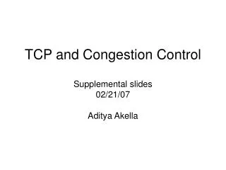
Hybrid Modeling of TCP Congestion Control. Jo ã o P. Hespanha, Stephan Bohacek, Katia Obraczka, Junsoo Lee University of Southern California. Background. TCP/IP Transmission Control Protocol/Internet Protocol WWW, Telnet, FTP UNIX, Windows 98, Windows 2000 all include TCP/IP

E N D
Hybrid Modeling ofTCP Congestion Control João P. Hespanha, Stephan Bohacek,Katia Obraczka, Junsoo Lee University ofSouthern California
Background • TCP/IP • Transmission Control Protocol/Internet Protocol • WWW, Telnet, FTP • UNIX, Windows 98, Windows 2000 all include TCP/IP • The evolution of TCP/IP is supported by Internet Engineering Task Force(IETF) • Window based congestion control • If congestion occurs reduce sending rate to half, otherwise increase window size by 1 for each round trip time
Congestion control in data networks sources destinations B Congestion control problem: How to adjust the sending rates of the data sources to make sure that the bandwidth B of the bottleneck link is not exceeded? B is unknown to the data sources and possibly time-varying
Congestion control in data networks queue (temporary storage for data) r1 bps r2 bps rate ·B bps q(t)´ queue size r3 bps Congestion control problem: How to adjust the sending rates of the data sources to make sure that the bandwidth B of the bottleneck link is not exceeded?
Congestion control in data networks queue (temporary storage for data) r1 bps r2 bps rate ·B bps q(t)´ queue size r3 bps When åi ri exceeds B the queue fills and data is lost (drops) )drop(discrete event) Event-based control: The sources adjust their rates based on the detection of drops
Window-based rate adjustment wi(window size) ´ number of packets that can remain unacknowledged for by the destination source i destination i e.g., wi = 3 t0 1st packet sent t1 2nd packet sent t2 t0 3rd packet sent 1st packet received & ack. sent t1 2nd packet received & ack. sent t2 t3 1st ack. received )4th packet can be sent 3rd packet received & ack. sent t t wi effectively determines the sending rate ri: round-trip time
Window-based rate adjustment queuegets full longerRTT ratedecreases queuegets empty negative feedback wi(window size) ´ number of packets that can remain unacknowledged for by the destination per-packet transmission time ´sending rate total round-trip time propagationdelay time in queueuntil transmission This mechanism is still not sufficient to prevent a catastrophic collapse of the network if the sources set the wi too large
TCP Reno congestion control • While there are no drops, increase wiby 1 on each RTT • When a drop occurs, divide wiby 2 (congestion controller constantly probe the network for more bandwidth) Network/queue dynamics Reno controllers drop detected(one RTT after occurred) ß ß drop occurs disclaimer: this is a simplified version of Reno that ignores some interesting phenomena…
Switched system model for TCP queue-not-full transition enabling condition (drop occurs) queue-full (drop detected) state reset
Switched system model for TCP queue-not-full s = 1 (drop occurs) queue-full (drop detected) s = 2 alternatively… continuous dynamics discrete dynamics reset dynamics s2 {1, 2}
Linearization of the TCP model Time normalization´ define a new “time” variable t by 1 unit of t´ 1 round-trip time In normalized time, the continuous dynamics become linear queue-not-full queue-full
Switching-by-switching analysis x1 x2 T t0 t1 t2 t3 t4 t5 t6 queue-not-full queue full queue-not-full queue full queue-not-full queue full ´kth time the system enters the queue-not-full mode queue-not-full x1 x2 impact map queue-full state space
Switching-by-switching analysis x1 x2 T t0 t1 t2 t3 t4 t5 t6 queue-not-full queue full queue-not-full queue full queue-not-full queue full ´kth time the system enters the queue-not-full mode Theorem. The function T is a contraction. In particular, • Therefore • xk!x1 as k!1x1´ constant • x(t) !x1 (t) as t!1x1(t) ´ periodic limit cycle
NS-2 simulation results N1 Flow 1 S1 N2 Flow 2 S2 Bottleneck link TCP Sinks TCP Sources Router R2 Router R1 20Mbps/20ms S7 Flow 7 N7 window size w1 S8 N8 Flow 8 window size w2 window size w3 window size w4 window size w5 window size w6 window size w7 window size w8 queue size q 500 400 300 Window and Queue Size (packets) 200 100 0 0 10 20 30 40 50 time (seconds)
Results t0 t1 t2 t3 t4 t5 t6 queue-not-full queue full queue-not-full queue full queue-not-full queue full Window synchronization: convergence is exponential, as fast as .5k Steady-state formulas: average drop rate average RTT average throughput
What next? queue-not-full r1 bps queue r2 bps B bps queue-full r3 bps Other models for drops: • One drop per flow is very specific to this network: • all flows share the same queue • similar propagation delays for all flows • constant bit-rate cross traffic • “drop-tail” queuing discipline
What next? Other models for drops: How many drops? qmax # of drops ´ squeue-full(inrate outrate) q(t) t queue full queue-not-full number of packets that are out for flow i Which flows suffer drops? total number of packets that are out This probabilistic hybrid model seems to match well with packet-level simulations, e.g., with drop-head queuing disciplines. Analysis ???
What next? More general networks: qB flow 1 qC flow 2 qA qD flow 3
What next? More general networks: qB flow 1 qC flow 2 qA qD flow 3 portion of the queue due to flow i total queue size drop occurs outgoing rate of flow i
What next? More general networks: qB flow 1 qC flow 2 qA qD flow 3 ß drop occurs
What next? Even multicast (current work)… qB flow 1 qC flow 2 qA qD ß drop occurs
Conclusions • Hybrid systems are promising to model network traffic in the context of congestion control: • retain the low-dimensionality of continuous approximations to traffic flow • are sufficiently expressive to represent event-based control mechanisms Hybrid models are interesting even as a simulation tool for large networks for which packet-by-packet simulations are not feasible Complex networks will almost certainly require probabilistic hybrid systems
Switching-by-switching analysis queue-not-full xk xk+1 impact map queue-full state space Impact maps are difficult to compute because their computation requires: Solving the differential equations on each mode (in general only possible for linear dynamics) Intersecting the continuous trajectories with a surface(often transcendental equations) It is often possible to prove that T is a contraction without an explicit formula for T…