Download
1 / 87
870 likes | 918 Views
So far we can compare 2 groups/conditions and assess 1 dependent variable E.g., 1 group seeing pictures of and 1 group seeing real spiders (independent variable); measuring their level of anxiety (dependent var)

E N D
So far we can compare 2 groups/conditions and assess 1 dependent variable E.g., 1 group seeing pictures of and 1 group seeing real spiders (independent variable); measuring their level of anxiety (dependent var) If we want to compare more than 2 groups/ conditions and assess 1 dep var, we have to use an Analysis of Variance (ANOVA) Chapter 8 is about independent ANOVA, i.e, where the various groups/conditions consist of different subjects Chapter 8_Field_2005: Comparing several means: ANOVA (General Linear Model, GLM 1)
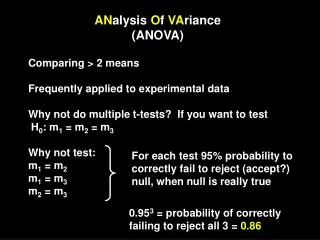
Suppose we had 3 groups – why not carry out 3 independent t-tests between those 3? because the probability p of making Type 1 error rises dramatically Remember: for 1 test, the p of not making any Type 1 error is = .95. For 3 tests, this p is .95 x .95 x .95 = .857 Hence, the p of committing a Type 1 error is 14.3%! Even worse for more groups! The problem: experimentalwise error rate G 1 G1 -G2 G 2 G1 -G3 G 3 G2 -G3
ANOVA gives us an overall F-value that tells us whether n means are the same, in an overall test (omnibus test). It looks for an overall experimental effect. It does NOT tell us which of the group differences cause this overall effect, only that X1 = X2 = X3 is NOT true. Separate contrasts may be carried out later The solution: ANOVA
Experimental research Conducted controlled experiments Had adopted ANOVA ANOVA as regresssion • Correlational research • Looked at real-world relationships • Had adopted multiple regression Although having arisen in different research contexts, regression and ANOVA are conceptually the same thing! The General Linear Model (GLM) accommodates this fact.
ANOVA compares the amount of systematic variance to the unsystematic variance. This ratio is called F-ratio: ANOVA: F-ratio: systematic (experimental) variance unsystematic (other and error) variance Regression: F-ratio: variance of the regression model variance of the simple model ANOVA as regression
The F-ratios in ANOVA and regression are the same. ANOVA can be represented by the multiple regression equation with as many predictors as the experiment has groups minus 1 (because of the df's) ANOVA as regression
We compare 3 independent groups Indep Var (IV): treating subjects with 'Viagra' 1. placebo 2. low dose of V 3. high dose of V Dep Var (DP): measure of 'libido' General equation for predicting libido from treatment Outcomei= (Modeli) + errori In a regression approach, the 'experimental model' and the 'simple model' were coded as dummy variabes (1 and 0). The outcome of the good model was compared to that of the simple model. An example (using viagra.sav)
With more than two groups, we have to extend the number of dummy variables in regression. If there are only 2 groups, we have a base category 0 and a real model 1. If there are more than 2 groups, we need as many coding variables as there are groups – 1. One group acts as a 'baseline' or 'control group' (0) In the viagra example, there are 3 groups, hence we need 2 coding variables (for the groups 'lw dose' and 'high dose') + a control group ('placebo') Dummy variables for coding groups
(8.2) Libidoi = b0 + b2Highi + b1Lowi + i A person'si libido can be predicted from knowing his group membership + the intercept b0. Equation for the Viagra-expl Outcome Variable Intercept = constant where the regression line cuts the y-axis =mean of placebo group Regression coefficient for the high group the comparison between the 2nd group and the placebo group Regression coefficient for the low group: comparison between the 1st group and the placebo group Error Note that we do not choose the overall mean (grand mean) as a base model (b0) but the mean of the control group, the placebo group.
So far, in linear regression we had chosen the grand mean as the base model. In binary logistic regression we had chosen the most frequent case as the base model. Here, we choose the placebo group as our base model (b0). Why, do you think? Choice of b0 – the constant This is because as good experimenters we have to control for any unspecific effects due to giving subjects any treatment. This we test with the placebo group. The comparison between the placebo and the experimental groups will tell us whether, above this unspecific effect, the drug (in various doses) has a causal effect on the dep var. Note that in regression you are free to choose your base model! That makes regression a highly flexible method.
Dummy coding of the 3 groups • Each group is now individuated by its particular code • Why can't we call the 3 groups: 0,1, 2, or 1,2,3? Because in regression we use these dummy variables in the regression equation when we set the groups to 0 or 1
Libidoi = b0 + (b2 x 0) + (b1x 0)i Libidoi = b0 XPlacebo = b0 The predicted value for the placebo group is its mean. This is the intercept/ constant (b0) against which we will test the two experimental groups. Equation for the Placebo group
Libidoi = b0 + (b2 x 1) + (b1x 0)i Libidoi = b0 + b2 XHigh = XPlacebo + b2 b2 = XHigh - XPlacebo The predicted value for the high-dose group is its mean. We compare this mean against the mean of the placebo group. b2 represents the difference between the two groups. Equation for the High-dose group
Libidoi = b0 + (b2 x 0) + (b1x 1)i Libidoi = b0 + b1 XLow = XPlacebo + b1 b1 = XLow - XPlacebo The predicted value for the low-dose group is its mean. We compare this mean against the mean of the placebo group. b1 represents the difference between the two groups. Equation for the low-dose group
In dummy.sav the three groups (in the column 'dose') are coded with two binary dummy variables (in the columns 'dummy 1' and 'dummy 2'), suited for multiple regression Multiple regression (using dummy.sav)
In dummy.sav, the Viagra data of the 3 groups are coded with dummy variables (0/1) as predictors Multiple regression (using dummy.sav) Coefficients The constant/intercept is the mean of the baseline group 'Placebo' b0 is already significant! b2 is significant: The difference between the 2 groups (placebo vs. High-dose) is sign. For the high-dose group, b2 is 5 – 2.2 = 2.8 b1 is n.s: The difference between the 2 groups (placebo vs. low-dose) is n.s. In a regression analysis the t-tests for the beta-coefficients are equal to group comparisons For the low-dose group, b1 is 3.2 – 2.2 = 1
Coding dummy-variables for arbitrary group contrasts For 4 groups, you need n-1 (4-1) = 3 dummy variables (DV's). The baseline group is coded 0 throughout.
In regression, the F-ratio tests the overall fit of a regression model to a set of observed data The same logic applies in ANOVA: we want to test if the means of n groups – in the Viagra example, 3 groups – are different. Thus, the Null-hypothesis is: all means are equal (i.e., they all equal the 'grand mean'.) The F-ratio Output from Multiple regression with dummy.sav
The Viagra data, graphically • B1: difference between 'placebo – low dose', n.s. • B2: difference between 'placebo – high dose', * • The Null-hypothesis is rejected: there are differences between the groups (due to the significant b2) Libido b2* b1 n.s. Subject (n=15)
The grand mean represents the case when all groups are equal (H0). If the groups do not differ, the data will all cluster around the grand mean If the b-values of the groups do differ, the regression line will differ from the grand mean. This regression line will represent the data better (H1) The regression model will explain some variance and leave some variance unexplained: F ratio: systematic (experimental) variance unsystematic (other and error) variance The amount of explained variance is bigger than the amount of unexplained variance The logic of ANOVA
(8.3) Deviation = (observed – model)2 With equation (8.3) we calculate the fit of the basic model (placebo group, b0) and the fit of the best model (regression model, b1 and b2). If the regression model is better than the basic model, it should fit the data better, hence the deviation between the observed data and the predicted data will be smaller. Basic equation
For all data points, we sum up their differences from the grand mean and square them. This is SST. (8.4) SST = (xi – xgrand )2 The grand variance is the SST/(N-1). From the grand variance we can caculate the SST. Total sum of squares (SST)
SST = s2grand (n-1) = 3.124 (15-1) = 3.125 x 14 = 43.74 Calculating SST from the grand variance Grand Variance
For any number of observations, the degrees of freedom is (n-1) since you can only choose (n-1) values freely, whereas the last obervation is determined – it is the only one that is left. If we have 4 observations, they are free to vary in any way, i.e., they can take any value. If we use this sample of 4 observations to calculate the SD of the population (i.e., SE), we take the mean of the sample as an estimate of the population's mean. In doing so, we hold 1 parameter (the mean) constant. Degrees of freedom, df
If the sample mean is 10, we also assume that the population mean is 10. This value we keep constant. With the mean fixed, our observations are not free to vary anymore, completely. Only 3 can vary. The fourth must have the value that is left over in order to keep the mean constant Expl: If 3 observations are 7,15, and 8, then the 4th must be 10, in order to arrive at a mean of 10. Thus, holding one parameter constant, the df are one less than the N of the sample, df = n-1 Therefore, if we estimate the SD of the population (SE) from the SD of the sample, we divide the SS by n-1 and not by n. Degrees of freedom, df – continued
The overall variance is SST = 43.74 Now we want to know how much of this variance is 'model' variance SSM, i.e., can be explained by the variation between the three groups. For each participant, the predicted value is the mean of its condition, i.e., 2.2 for the placebo group, 3.2 for low dose and 5 for high dose. The difference of these predicted values from the grand mean are calculated, squared, multiplied by the n in each group and summed up in SSM. 5 3.2 2.2 Model Sum of Squares SSM Grand mean
SSM = nk(xk – xgrand)2 SSM = 5(2.2 – 3.467)2 + 5(3.2 – 3.467)2 + 5(5 – 3.467)2 = 5(-1.267)2 + 5(-0.267)2+ 5(1.533)2 = 8.025 + 0.355 + 11.755 = 20.135 The df of SSM is the number of parameters k (3 groups) minus 1 = 3-1=2 N of subjects in each group Calculating SSM Placebo group Low dose group High dose group
We know already: SST = 43.74 and SSM = 20.14 SSR = SST - SSM SSR = 23.6 Residual Sum of Squares SSR
For nerds: calculating the Residual Sum of Squares SSR properly SSR =xik- xk)2
SSR =( xik– xk)2 This equation is identical to: SSR= SSgroup1 + SSgroup2 + SSgroup2 SSR = s2k (nk - 1) For nerds: calculating the Residual Sum of Squares SSR properly Variance for each group k Number of participants in each group
SSR = s2k (nk - 1) SSR= (1.7) (5-1) + (1.7) (5-1) + (2.5) (5-1) = 6.8 + 6.8 + 10 = 23.60 For nerds: calculating the Residual Sum of Squares SSR properly DfR = dfT – dfM = 14 – 2 =12
MS is the SS divided by the df MSM = SSM = 20.135 = 10.067 dfM 2 MSR = SSR = 23.60 = 1.967 dfR 12 Average amount of Variation explained by the model - systematic variation Mean squares MS (average SS) Average amount of Variation not explained by the model - unsystematic variation
The F-ratio is the ratio between the systematic (explained) and unsystematic (unexplained) variable: F = MSM MSR Commonsense logic: If F < 1, then the t-test must be n.s. since then the unsystematic variance MSR is bigger than the systematic variance MSM. F-ratio
F = MSM = 10.067 = 5.12 MSR 1.967 In order to know if 5.12 is significant* we have to test it against against the maximum value we would expect to get by chance alone look up F-distribution, Appendix A.4 ( p 756) with a df=2 (numerator) and df=12 (denominator) , we find a criticial value of 3.89 (p = .05) and 6.93 (p = .01) the F-ratio is * on the 5%-level F-ratio for Viagra data
How robust is ANOVA? Homogeneity: Robust when sample sizes are equal Very sensitive to dependent observations Interval scale:Robust even with dichotomous variables, but df should be high (20) Assumptions of ANOVA Same assumptions as for any parametric test: • Normal distribution • Homogeneous variances • observations should be independent • Interval scale level
The F-ratio is a global ratio and tells us whether there is a global effect of the experimental treatment, BUT, if the F-value is significant *, it does NOT tell us which differences (b-coefficients) made the effect significant. It could be that b1 or b2 or both are * Thus, we need to inquire further Planned contrasts – post hoc tests Planned comparisons Post hoc tests or
In 'planned contrasts' we break down the overall variance into component parts. It is like conducting a 1-tailed test, i.e., when you have a directed hypothesis. Expl. Viagra: 1st contrast: two drug conditions > placebo 2nd contrast: high dose > low dose 1. Planned contrasts
Partitioning SSM ANOVA SST (43.73) Total variance in data SSM (20.13) Systematic variance SSR (23.6) Unsystematic variance SSM (20.13) Systematic variance 1st contrast Low + high dose Variance explained by experimental groups Placebo Variance explained by control 2nd contrast For comparing 'low dose' vs placebo, we need to carry out a post-hoc test! Low dose High dose
Planned contrasts are like slicing up a cake: once you have cut out one piece, it is unavailable for the next comparison (k-1) contrasts: The number of contrasts is always one less than the number of groups Each contrast compares only 2 chunks of variance The first comparison should always be between all the experimental groups and the control group(s) Rationale of planned contrasts SSM High dose SSR Low dose Placebo
SSM Variance explained by experiment Four groups: E1, E2, E3, and C1 Contrast 1 Control group C1 Experimental groups E1,2,3 Contrast 2 E1 and E2 E3 Planned comparisons in an experiment with 3 Exp and 1 C group Contrast 3 E1 E2
SSM Variance explained by experiment Four groups: E1, E2 and C1, C2 Contrast 1 Control groups C1and C2 Experimental groups E1and E2 Contrast 2 E1 E2 Planned comparisons in an experiment with 2 Exp and 2 C- groups Contrast 3 C1 C2
In a planned contrast, we compare 'chunks of variance'. Each chunk can represent more than one group When we carry out contrasts, we assign values to the dummy variables in the regression model With the values we specify which groups we want to compare The resulting coefficients (b1, b2) represent the comparisons The values are called weights We compare any group with a positive weight against any group with a negative weight Carrying out contrasts
Rule 1: Choose sensible comparisons. Rule 2: One chunk of variation is coded with a positive value; the other chunk with a negative value. Rule 3: The sum of weights in a contrast is 0. Rule 4: A group that is not included in the contrast is coded as 0. It does not participate in the contrast Rule 5: The weights assigned to the group(s) in one chunk of variation should be equal to the number of groups in the oppositive chunk of variation Rules for carrying out contrasts
Weights for the Viagra Expl, 1st contrast SSM (20.13) Systematic variance Placebo Low + high dose Rule 2: Positivesign of weight negative each 1magnitude of weight 2 Rule 5: +1+1weight -2 Rule 3: +1 + +1 weights = 0 + -2 = 0
Weights for the Viagra Expl, 2nd contrast Chunk 1 Low dose Chunk 2 High dose Placebo not included Rule 2: Positivenegative sign of weight -- 1 1 magnitude of weight 0 Rule 5: +1- 1weight 0 Rule 3: +1 +- 1 weights = 0 0
(8.9) Libidoi = b0 + b1Contrast1 + b2Contrast2 NOW B0 represents the grand mean B1 represents contrast1 (exp groups vs. Placebo) B2 represents contrast2 (low vs. High dose) Regression equation for coding of contrasts Again, you see that you may choose your base model (b0) freely, according to a given model that you want to test
Orthogonal contrasts for Viagra Expl • Important: • All sums (total),over each variable and over the Product of the contrasts, have to be 0! • This means that the contrasts are independent of each other, i.e., orthogonal (in a 90° angle) • Independence prevents the error in the t-test to inflate!
The intercept (b0) is equal to the grand mean: b0 = grand mean = (XHigh + XLow + Xplacebo)/3 For nerds: dummy coding and regression
Libidoi = b0 + b1Contrast1 + b2Contrast2 XPlacebo= XHigh+XLow +XPlacebo + (-2b1) + (b2 x 0) 3 Regression equation, using the contrast codes of the first contrast -2 for contrast 1 0 for contrast 2