Download
1 / 55
550 likes | 691 Views
Chapter 13 Scheduling Groups of Jobs. 2013 년 2 학기 스케줄이론 (406.653) Prof. Jinwoo Park. Contents. 1. Introduction 2. Scheduling Job Families 2.1. Minimizing Total Weighted Flow Time 2.2. Minimizing Maximum Lateness 2.3 . Minimizing Makespan in the Two-Machine Flow Shop

E N D
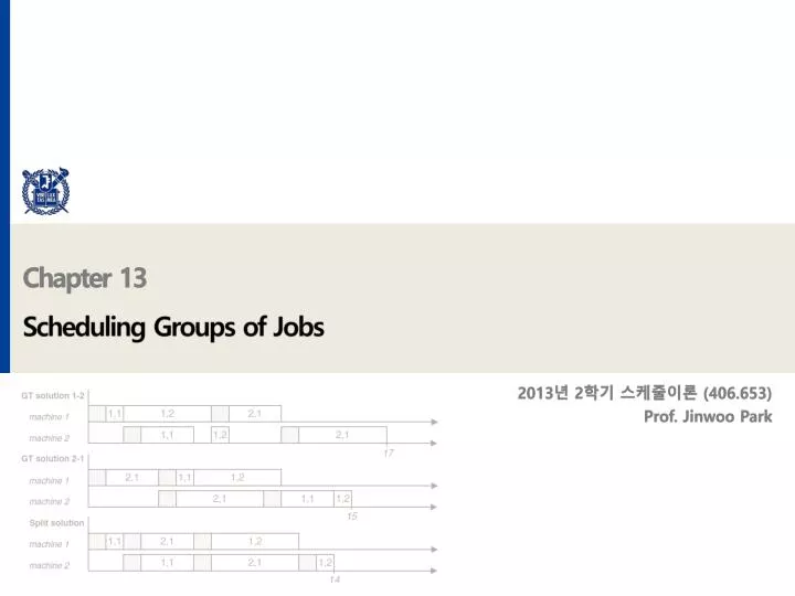
Chapter 13Scheduling Groups of Jobs 2013년 2학기 스케줄이론(406.653) Prof. Jinwoo Park
Contents 1. Introduction 2. Scheduling Job Families 2.1. Minimizing Total Weighted Flow Time 2.2. Minimizing Maximum Lateness 2.3. Minimizing Makespan in the Two-Machine Flow Shop 3. Scheduling with Batch Availability 4. Scheduling with a Batch Processor 4.1. Minimizing the Makespan with Dynamic Arrivals 4.2. Minimizing Makespan in the Two-Machine Flow Shop 4.3. Minimizing Total Flowtime with Dynamic Arrivals 4.4. Batch-Dependent Processing Times 5. Summary
Introduction • Grouping of jobs result in better resource utilization. • Basically two types of Grouping exist: • Family Scheduling Model (sharing common set-up) • Batch Processing Model (processor characteristic)
Scheduling Job Families • Let us use the pair (i,j) to refer to job j of family i, and let f denote the number of families, n the number of jobs, and nithe number of jobs belonging to family i. • DefinitionGT (group technology) assumption: precisely one and only one setup for each family in a given planning period. • The makespan is minimal in a GT solution, because additional setups would only make the makespan greater. Moreover, in a GT solution the makespan is a constant independent of sequence. Let pi denote the total processing time for family i, or . • Then the makespan for a GT solution is given by
Minimizing Total Weighted Flow Time • Theorem 13.1In the F-problem under the GT assumption, the jobs within a family should be scheduled according to SPT, and the families should be scheduled in non-decreasing order of . • Theorem 13.2In the FW-problem under the GT assumption, the jobs within a family should be scheduled according to SWPT, and the families should be scheduled in non-decreasing order of . • Theorem 13.3In the FW-problem for the family scheduling model, suppose all jobs in each family have identical processing times and weights. Then there exists an optimal solution that is a GT solution. Show Proof Show Proof Show Proof
Minimizing Maximum Lateness • Theorem 13.4In the Lmax-problem under the GT assumption, the jobs within a family should be scheduled according to EDD. Then the families should be ordered by EDD, using family due dates scheduled in non-decreasing order of. • Theorem 13.5In the Lmax-problem for the family scheduling model, suppose all jobs within a family have identical due dates. Then there exists an optimal solution that is a GT solution. Show Proof Show Proof
Minimizing Makespan in the Two-Machine Flow Shop • An algorithm similar to Jonhnson's rule can be applied.
Scheduling with Batch Availability • Theorem 13.6In the F-problem with batch availability and one family, there is an optimal schedule in which the jobs appear in non-decreasing order of their processing times. • Theorem 13.7In the F-problem with batch availability and one family, the batch sizes form a non-increasing sequence. Show Proof Show Proof
Minimizing the Makespan with Dynamic Arrivals • ERT(Earliest Ready Time) and FOE(First-Only-Empty) algorithm. • Algorithm 13.1The FOE algorithm • Theorem 13.8In the batch processor scheduling model, the FOE algorithm produces the minimum makespan. Show Proof
Minimizing Makespan in the Two-Machine Flow Shop • Example 13.6two machine 18 job scheduling problem. • Consider the problem of scheduling n = 18 jobs on two machines. The jobs have the following characteristics. • From (13.7), and considering k = 1, 2, . . . , 6, we have
Minimizing Total Flowtime with Dynamic Arrivals • Similar to two machine case.
Batch-Dependent Processing Times • DP formulation
Summary • Two types of scheduling models involving groups of jobs.
Chapter 13 - AppendixScheduling Problem in Steel Industry 2013년 2학기 스케줄이론 (406.653) Prof. JinwooPark & Lee HyoungGon
Synchronized Scheduling Method in Manufacturing Steel Sheets RYOJI TAMURA1, MEGUMI NAGAI1 1Information Systems Department, Sumitomo Metal Industries, Fukuoka. International Federation of Operational Research Societies (IFORS) Vol. 5, No. 3, 1998, pp. 189~199
Introduction • New Scheduling System • Casting to a rolling process in steel sheets manufacturing • Multi-objective assigning and sequencing problem with lots of constraints • Two-Stage algorithm composed of macro-scheduling and micro-scheduling.
Steel Sheets Manufacturing Process Cast-to-roll scheduling problem
Primary Production Scheduling at Steelmaking Industries H.S. Lee 1, S.S. Murthy 1 1IBM Research Division, Thomas J. Watson Research Center, P.O. Box 218, Yorktown Heights, New York 10598, USA. IBM Journal of Research and Development Vol. 40, No. 2, 1996, pp. 231~252.
Overview of steelmaking and the primary steelmaking process (1/2) • Iron making • Combining the raw ingredients of steel into a generic intermediate product known as hot iron or pig iron. • Primary steelmaking • Accepts the supply of hot iron from the blast furnace and transforms it into semi-finished products in a variety of grades(specific metallurgical compositions of steel), shapes, and dimensions.
Overview of steelmaking and the primary steelmaking process (2/2) • Finishing • Consists of numerous operations that can be applied selectively to the semi-finished products of the primary steelmaking process, to achieve customers’ specifications • Cold-rolling ⇒ precise dimension, surface finish, mechanical property • Annealing : material’s grain size, ductility • Tempering: internal stresses, ductility • Pickling: clean the surface • Coatings: corrosion resistance
Scheduling issues in primary steel production • Utilization of manufacturing units • Allocation of production among parallel manufacturing • Specification of heats or heat groups • Specification of rolling groups • Sequencing of heats/rolling groups for manufacturing • Coordination of schedules between production stages • Rescheduling
Scheduling for continuous casters (1/3) • Simple mixed-integer linear programming model • “A model for sequencing a continuous casting operation to minimize costs”(1987) • Electric arc furnace, no change of width in continuous casters, single objective cost function
Scheduling for continuous casters (2/3) • Complex models using heuristics(LTV caster scheduling model) • Implemented in 1983, in support of the first continuous caster installed at LTV Cleveland Works. • Maximization of on-time delivery • Maximization of caster productivity • Satisfaction of quality requirements • Minimization of semifinished inventory • “A Scheduling Model for LTV Steel’s Cleveland Work’s Twin-Strand Continuous Slab Caster”(1988) • “Twin Strand Continuous Slab Caster Scheduling Model”(1990)
Scheduling for continuous casters (3/3) • Cooperative scheduling approach in which an expert system assists a scheduler(Scheiker Scheduling) • “Cooperative scheduling and its application to steelmaking processes”(1991) • Iteratively modifies an existing schedule through the user interface • Scheduler typically makes global changes that increase global efficiency • Scheduling engine uses a rule base to recognize violations of local constraints
Scheduling for hot strip mill • “Roll-A-Round program”(1991) • Uses heuristics based on the traveling-salesman problem and linear programming
(Back to…) Synchronized Scheduling Method in Manufacturing Steel Sheets RYOJI TAMURA1, MEGUMI NAGAI1 1Information Systems Department, Sumitomo Metal Industries, Fukuoka. International Federation of Operational Research Societies (IFORS) Vol. 5, No. 3, 1998, pp. 189~199
Steel Sheets Manufacturing Process (2/2) • “heat”: necessary amount of molten steel to be poured into the BOF once. • “try”: the molten steel is poured 5-7times consecutively, and this sequence of heat is called a “try”. • “chance”: rolls are exchanged after rolling one try amount of slabs, and this exchange interval is called a “chance”. • Thus one “try” in casting corresponds to one “chance” in rolling.
The Problem(1/3) - Three Main Objectives • To incorporate particular instructed orders/slabs into the schedule • To attain the target supply quantity for subsequent processes • To meet the rolling due-date
The Problem(2/3) - Constraints • Cast Constraints • The same ingredient orders must be gathered • The “first” heat requires about 270 tons • The last slab of a “try” requires low grade order • Roll Constraints • The strip width has to be changed from wider to narrower • The strip thickness should be transmitted smoothly • Particular orders requires positional limits in rolling sequence • Etc….
The Problem(3/3) - Conventional scheduling • 24 hours, 5-7 roll “chances”, three shifts of workers(4) • Select and sequence 60-80 pieces among 5000 orders per roll chance • Consecutively, select 50-70 pieces among 3000 non-D/C slabs in the yard, and insert them between orders. • Some know-how is established to some extent, but for the most part it depends upon a trial-and-error method.
The reason of taking the two-stage approach • Main reason • Reduction of computing time by avoiding combinatorial explosion. • Following advantages • Creating a balanced schedule to avoid differences from the expected one. • Improving solution precision and easiness to check the schedule by user participability • Program flexibility for environmental changes.
Macro Scheduling • Generating a feasible route. • - feasible block sequence. • Pseudo-assignment of slabs to the route. • Repetition for all feasible routes. • Determination of the optimum route.
Micro Scheduling Selecting a block on the route. Selecting a previous path sequence. Generating a feasible path. Pseudo-assignment of slabs to the path. Linking a path to the previous path sequence and evaluating the new path sequence. Repetition for all feasible paths. Repetition for all previous path sequences. Reduction of the path sequences. Repetition of all blocks. Determination of the optimum sequence and assignment of slabs.
User Interface • Preparation • Operators can refer to necessary information(order, slab spec, input parameter) • Modification • Refine the schedule(insert slabs, delete slabs or exchange the slab position)
Conclusion • Human-machine harmonization scheduling system. • Now this system largely contributes to efficient scheduling, in Kashima Steel Works.
Q n A TA 석사과정 전성범 junsb87@mailab.snu.ac.kr
Theorem 13.1 Go back
Theorem 13.2 Go back
Theorem 13.3 Go back
Theorem 13.4 Go back
Theorem 13.5 Go back