Download
1 / 64
650 likes | 825 Views
SAT -based Bounded and Unbounded Model Checking. Edmund M. Clarke Carnegie Mellon University. Joint research with C. Bartzis, A. Biere, P. Chauhan, A. Cimatti, T. Heyman, D. Kroening, J. Ouaknine, R. Raimi, O. Strichman, and Y. Zhu. Why am I giving this talk?.

E N D
SAT-based Bounded and Unbounded Model Checking Edmund M. Clarke Carnegie Mellon University Joint research with C. Bartzis, A. Biere, P. Chauhan, A. Cimatti, T. Heyman, D. Kroening, J. Ouaknine, R. Raimi, O. Strichman, and Y. Zhu
Why am I giving this talk? I have an ulterior motive for this talk. Second Edition! Need a chapter on SAT for the second edition.
Outline of Talk 1. Motivation 2. Bounded Model Checking 3. Complete methods using SAT a. Induction b. Unbounded Model Checking --- with cube enlargement --- with circuit co-factoring --- with interpolants
Outline of Talk 1. Motivation yes 2. Bounded Model Checking yes 3. Complete methods using SAT a. Induction no b. Unbounded Model Checking --- with cube enlargement yes --- with circuit co-factoring yes --- with interpolants no
Model Checking (CE81,QS82) • Specification – temporal logic • Model – finite state transition graph • Advantages: • Always terminates • Automatic • Usually fast • Can handle partially specified models • Counterexample if specification is false
Symbolic Model Checking • Method used by most “industrial strength” model checkers. • Uses Boolean encoding for state machine and sets of states. • Can handle much larger designs – hundreds of state variables. • BDDs traditionally used to represent Boolean functions.
Problems with BDDs • BDDs are a canonical representation. Often become too large. • Variable ordering must be uniform along paths. • Selecting right variable ordering very important for obtaining small BDDs. • Often time consuming or needs manual intervention. • Sometimes, no space efficient variable ordering exists. This talk describes alternative approaches to model checking that use SAT procedures.
Advantages of SAT Procedures • SAT procedures also operate on Boolean formulas but do not use canonical forms. • Do not suffer from the potential space explosion of BDDs. • Different split orderings possible on different branches. • Very efficient implementations exist.
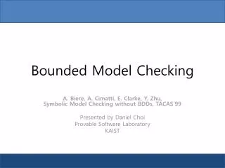
Bounded Model Checking A. Biere, A. Cimatti, E. Clarke, Y. Zhu, Symbolic Model Checking without BDDs, TACAS’99
Bounded Model Checking as SAT Given a propertyp: (e.g. “signal_a = signal_b”) Is there a state reachable inkcycles, which satisfiesp? p p p p p . . . s0 s1 s2 sk-1 sk
Bounded Model Checking: Safety The reachable states in k steps are captured by: The property p fails in one of the k steps
Bounded Model Checking: Safety The safety propertypis valid up to stepk iffW(k)is unsatisfiable: p p p p p . . . s0 s1 s2 sk-1 sk
11 00 10 01 Bounded Model Checking: Safety Example: a two bit counter Initial state:I: :l^:r Transition:R: l’ = (lr) ^r’ = :r Property:G(l r). Fork = 2, W(k)is unsatisfiable. Fork = 3 W(k)is satisfiable
Bounded Model Checking: Liveness There is no counterexample of lengthkto the Liveness propertyFpiffW(k)is unsatisfiable: = p :p :p :p :p . . . s0 s1 s2 sk-1 sk
k l i BMC formula for arbitrary LTL(Standard translation) Size of resulting formula: O(k|M| + k3||) With sharing of subformulas becomes O(k|M| + k2||)
A fixpoint based translation • Idea: for lasso-shaped Kripke structures, the semantics of LTL and CTL coincide. • Add a formula that isolates a lasso-shaped path. • Use the fixpoint characterization of CTL, e.g. E[U ] = (^EX E[U ]) T. Latvala, A. Biere, K. Heljanko, and T. Junttila: “Simple Bounded LTL Model Checking” FMCAD 04 i k
LTL formula Model Isolate lasso-shaped path bound Fixpoint formula Overall formula
Loop constraints • If li is true then there exists a loop at position i. • At most one li is true.
Fixpoint formula k i j False True Size of resulting formula: O(k(|M| + ||))
Generating the BMC formula(Based on the Vardi-Wolper algorithm) • A labeled Büchi automaton is a 5-tuple B=hS, S0, , L, Fi • Acceptance condition: An infinite word w is accepted iff the execution of w on B passes through a final state an infinite number of times. states initial states transition relation labels final states
s0 LTL model checking • Given • Transition system M • LTL property • Translate into a Buchi automaton B • Compute product automaton P=M £B • Check if Pis empty: Is a fair loop reachable?
s0 Generating the BMC formula • Encode all paths ofP that start at an initial state and are k steps long. • Require that • at least one path contains a loop. • at least one state in the loop is final. E. Clarke, D. Kroening, J. Ouaknine, and O. Strichman: “Computational chalenges in Bounded Model Checking” STTT 05
s0 sl=sk sk-1 Generating the BMC formula Start from the initial state Require that some state in the loop is final Choose a state where the loop starts Follow k transitions
Resources exceeded SAT BMC(M,,k) yes k¸CT Bounded Model Checking k = 0 k++ UnSAT no CTis the completeness threshold
The Completeness Threshold • Computing CT is as hard as model checking. • Idea: Compute an over-approximation to the actual CT • Consider system Pas a graph. • Compute CTfrom structure of P.
DI(M)= RDI(M)= Basic notions • DiameterD(M)=longest shortest path between any two reachable states. • Recurrence DiameterRD(M)=longest loop-free path between any two reachable states. • The initialized versions:DI(M) and RDI(M)start from an initial state. D(M) = 2 RD(M) = 3
s0 p · DI(M) p p p p CT for safety properties • Theorem: forAGppropertiesCT = DI(M) ForAFpproperties this does not hold DI(M)=3 but CT=4
p p p p p s0 CT for liveness properties • Theorem: forAFppropertiesCT= RDI(M)+1 • Theorem: for an LTL propertyCT = ?
·dI(P ) ·d(P ) ·rdI(P ) s0 CT for arbitrary LTL properties Theorem [CKOS 05] A Completeness Threshold for any LTL property is min(rdI(P )+1, dI(P )+d(P )) Shortest counterexample
Why take the minimum? Example 1 dI(P)+d(P) = 6 rdI(P)+1 = 4 > Example 2 dI(P)+d(P) = 2 rdI(P)+1 = 4 <
State s is reachable in j steps: Thus, k is greater or equal to the diameter d if Formulation of diameter in QBF Infeasible to compute the diameterusing a poly-time algorithm for shortest paths.
SAT-based Diameter Computation • M. Mneineh, K. Sakallah,“SAT-based Sequential Depth Computation”,ASPDAC03 • Check if there is a state s reachable in c steps but not reachable in less than c steps. • Increment c, until no state is reachable in c steps. • May enumerate many states in 1.
Find maximal n that satisfies: Optimization: Use a sorting network to obtain an ordered permutation of the states [Kroening & Strichman] s0’ s0 comp & swap comp & swap s1’ s1 comp & swap s2’ s2 Now compare only neighboring states Recurrence diameter as SAT O(n2) O(nlogn) O(n)
Complexity of BMC: Formula size • Original translation O(k|M| + k2||) • Automata based translation O(k|M|2||) • Fixpoint based translation O(k(|M| + ||))
Complexity of BMC • Size of SAT instance is O(k(|M| + ||)) • k can become as large as the diameter of the system, which is exponential in the number of state variables in the worst case. • SAT is exponential time. • Therefore, SAT based BMC has doubly exponential complexity. • But LTL model checking is singly exponential!
Why use SAT based BMC? • Infeasible to represent P explicitly. • Identify shallow errors efficiently. • In many cases rd(P)and d(P)are not exponential and can be rather small. • E.g. hardware components without counters • Modern SAT solvers are very successful in practice.
Unbounded Model Checkingusing Cube Enlargement P. Chauhan, E. Clarke, and D. Kroening: “Using SAT based Image Computation for Reachability Analysis” CMU-CS-03-151
Reachability analysis • Consider a system with state variables x and inputs i. • S0(x) is the set of initial states. • T(x,i,x’) is the transition relation. • We want to compute the set of reachable statesSreach . • Iterative process: Compute the states reachable in 1 step, 2 steps, …
Image computation and Reachability • The set of immediate successors of states S(x) is given by: • The set of all reachable states is the least fixpoint: Img(S) = 9 x, i. T(x, i, x’) Æ S(x)
Computing Reachability • Si+1is the set of new states directly reachable from Si • Then Sreach is the union of all Si
SAT based image computation • The transition relation T(x,i,x’) is represented as a CNF formula (a set of clauses). • If not already in CNF, it can be converted in polynomial time. • The set of newly reachable states after each step Si as well as their union Sreach are represented in DNF (a set of cubes). • Obviously Sreach is in CNF.
Union of sets of cubes Si+1 contains all solutions to Si(x) T(x, i, x’) Sreach(x) projected on x’ and renamed to x SAT based image computation
The image computation step • Si is in DNF • Convert to CNF by introducing new variables • Solve the CNF formula Si(x) T(x,i,x’) Sreach(x) • Solution is a cube d • Project d to x’ and rename to x • Add d to Sreach(x) and Si+1(x) • Repeat until the formula becomes unsat
Efficiency issues • The number of satisfying assignments can be exponential in the number of variables. Therefore two problems: • Enumeration of full assignments is slow. • Solution: Cube enlargement • The representation of Sreach and Sican grow too large. • Solution: Systematically combine cubesusing an appropriate data structure.
Cube enlargement • SAT solvers like zChaff return complete assignments (minterms). • Partial assignments (cubes) are better, because they represent multipleminterms. • For example, the cube x1 x4 represents 4 minterms: • x1 x2 x3 x4 • x1 x2 x3 x4 • x1 x2 x3 x4 • x1 x2 x3 x4
Efficient cube set representation • Cubes are stored in a hash table of tries. • Each trie is associated to a unique subset of state variables. • Whenever a new cube d is inserted, the corresponding trie is searched for cubes d’ that differ only in one literal. • The merged cube (without the differing literal) is stored instead of d and d’.
{x2,x3,x4} Efficient cube set representation Hash table Hash keys {x1,x2} {x1,x7,x8} {x2,x4} … Tries {x2,x3,x4} • New cube:x2x3x4 • Identify appropriate hash table entry • Look for matching cubes • If match was found, delete cube and insert merged cube x2 x2 x3 x3 x4 x4 x2x4
Related work • [Gupta et al, FMCAD 00 and ICCAD 01] Mixed BDD / SAT approach • [K. McMillan, CAV 02] Sets of states represented in CNF CNF clauses stored in ZDDs Conflict analysis for cube enlargement • [H. Kang and I. Park, DAC 03] Offline Espresso to reduce the number of cubes No cube enlargement
Unbounded Model Checking using Circuit Cofactoring M. Ganai, A. Gupta and P. Ashar, “Efficient SAT-based Unbounded Symbolic Model Checking Using Circuit Cofactoring”, ICCAD 04