Download
1 / 56
560 likes | 562 Views
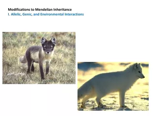
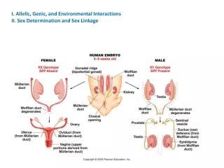
Explore the concepts of genetic linkage and inheritance patterns related to allelic, genic, and environmental interactions, sex determination, and sex linkage.

E N D
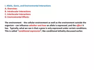
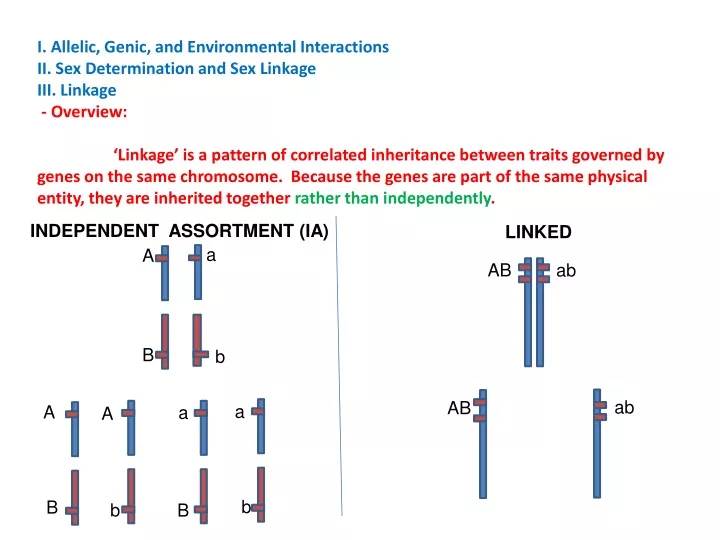
I. Allelic, Genic, and Environmental Interactions II. Sex Determination and Sex Linkage III. Linkage - Overview: ‘Linkage’ is a pattern of correlated inheritance between traits governed by genes on the same chromosome. Because the genes are part of the same physical entity, they are inherited together rather than independently. INDEPENDENT ASSORTMENT (IA) LINKED a A AB ab B b ab AB a A a A b B b B
III. Linkage - Overview: ‘Linkage’ is a pattern of correlated inheritance between traits governed by genes on the same chromosome. Because the genes are part of the same physical entity, they are inherited together rather than independently. Only ‘crossing-over’ can cause them to be inherited in new combinations. Cross-over products
III. Linkage A. ‘Complete’ Linkage - if genes are immediate neighbors, they are almost never separated by crossing over and are ‘always’ inherited together. The pattern mimics that of a single gene. AABB aabb AB ab X ab AB
III. Linkage A. ‘Complete’ Linkage - if genes are immediate neighbors, they are almost never separated by crossing over and are ‘always’ inherited together. The pattern mimics that of a single gene. AABB aabb AB ab X ab AB ab Gametes AB ab AB Double Heterozygote in F1; no difference in phenotypic ratios compared to IA F1
III. Linkage A. ‘Complete’ Linkage - if genes are immediate neighbors, they are almost never separated by crossing over and are ‘always’ inherited together. The pattern mimics that of a single gene. 1:1 ratio A:a 1:1 ratio B:b 1:1 ratio AB:ab Test cross X ab ab Phenotype Gametes ab AB ab AB ab AaBb AB – 50% aabb Ab – 50% Ab Aabb Ab If it was I.A., also: aB aaBb aB
III. Linkage A. ‘Complete’ Linkage B. ‘Incomplete’ Linkage
III. Linkage A. ‘Complete’ Linkage B. ‘Incomplete’ Linkage - Crossing over in a region is rare
III. Linkage A. ‘Complete’ Linkage B. ‘Incomplete’ Linkage - Crossing over in a region is rare - Crossing over events increase as the distance between genes increases A B C b c a LESS LIKELY IN HERE MORE LIKELY IN HERE
III. Linkage A. ‘Complete’ Linkage B. ‘Incomplete’ Linkage - Crossing over in a region is rare - Crossing over events increase as the distance between genes increases - So, the frequency of crossing over (‘CO’) gametes can be used as an index of distance between genes! (Thus, genes can be ‘mapped’ through crosses…) A B C b c a FEWER ‘CO’ GAMETES: Ab, aB MORE ‘CO’ GAMETES: bC, Bc
III. Linkage A. ‘Complete’ Linkage B. ‘Incomplete’ Linkage - Crossing over in a region is rare - Crossing over events increase as the distance between genes increases - So, the frequency of crossing over (‘CO’) gametes can be used as an index of distance between genes! (Thus, genes can be ‘mapped’ through crosses…) - How can we measure the frequency of recombinant (‘cross-over’) gametes? Is there a type of cross where we can ‘see’ the frequency of different types of gametes produced by the heterozygote as they are expressed as the phenotypes of the offspring?
TEST CROSS !!! III. Linkage A. ‘Complete’ Linkage B. ‘Incomplete’ Linkage b b A a a a B b
TEST CROSS !!! III. Linkage A. ‘Complete’ Linkage B. ‘Incomplete’ Linkage - So, since crossing-over is rare (in a particular region), most of the time it WON’T occur and the homologous chromosomes will be passed to gametes with these genes in their original combination…these gametes are the ‘parental types’ and they should be the most common types of gametes produced. b b A a a a B b a b A B
TEST CROSS !!! III. Linkage A. ‘Complete’ Linkage B. ‘Incomplete’ Linkage - Sometimes, crossing over WILL occur between these loci – creating new combinations of genes… This produces the ‘recombinant types’ b b A a a a B b a A b B a b A B
TEST CROSS !!! III. Linkage A. ‘Complete’ Linkage B. ‘Incomplete’ Linkage As the other parent only contributed recessive alleles (whether crossing over occurs or not)… b b A a b a a a b B a A B b a b A B
TEST CROSS !!! III. Linkage A. ‘Complete’ Linkage B. ‘Incomplete’ Linkage As the other parent only contributed recessive alleles (whether crossing over occurs or not)… SO: the phenotype of the offspring is determined by the gamete received from the heterozygote… b b A a a a B b a A b B a b A B
TEST CROSS !!! III. Linkage A. ‘Complete’ Linkage B. ‘Incomplete’ Linkage b b A a ALTERNATIVES ‘IA’ LINKAGE LOTS of PARENTALS FREQUENCIES EQUAL TO PRODUCT OF INDEPENDENT PROBABILITIES a a b B a A B b a b FEWER CO’S A B
III. Linkage • A. ‘Complete’ Linkage • B. ‘Incomplete’ Linkage • Example: • How do we discriminate between these two alternatives? • Conduct a Chi-Square Test of Independence AaBb x aabb
III. Linkage • A. ‘Complete’ Linkage • B. ‘Incomplete’ Linkage • Example: • How do we discriminate between these two alternatives? • Conduct a Chi-Square Test of Independence • - Compare the observed results with what you would expect if the genes assorted independently AaBb x aabb
III. Linkage • A. ‘Complete’ Linkage • B. ‘Incomplete’ Linkage • Example: • How do we discriminate between these two alternatives? • Conduct a Chi-Square Test of Independence • - Compare the observed results with what you would expect if the genes assorted independently AaBb x aabb The frequency of ‘AB’ should = f(A) x f(B) x N = 55/100 x 51/100 x 100 = 28
III. Linkage • A. ‘Complete’ Linkage • B. ‘Incomplete’ Linkage • Example: • How do we discriminate between these two alternatives? • Conduct a Chi-Square Test of Independence • - Compare the observed results with what you would expect if the genes assorted independently AaBb x aabb The frequency of ‘AB’ should = f(A) x f(B) x N = 55/100 x 51/100 x 100 = 28 The frequency of ‘Ab’ should = f(A) x f(B) x N = 55/100 x 49/100 x 100 = 27 The frequency of ‘aB’ should = f(a) x f(B) x N = 45/100 x 51/100 x 100 = 23 The frequency of ‘ab’ should = f(a) x f(b) x N = 45/100 x 49/100 x 100 = 22
III. Linkage • A. ‘Complete’ Linkage • B. ‘Incomplete’ Linkage • Example: • How do we discriminate between these two alternatives? • Conduct a Chi-Square Test of Independence • This is fairly easy to do by creating a contingency table: AaBb x aabb
III. Linkage • A. ‘Complete’ Linkage • B. ‘Incomplete’ Linkage • Example: • How do we discriminate between these two alternatives? • Conduct a Chi-Square Test of Independence • This is fairly easy to do by creating a contingency table: • Add across and down… • This gives the totals for each trait independently. AaBb x aabb
III. Linkage • A. ‘Complete’ Linkage • B. ‘Incomplete’ Linkage • Example: • How do we discriminate between these two alternatives? • Conduct a Chi-Square Test of Independence • This is fairly easy to do by creating a contingency table: • Then, to calculate an expected value based on independent assortment (for ‘AB’, for example), you multiple ‘Row Total’ x ‘Column Total’ and divide by ‘Grand Total’. • 55 x 51 / 100 = 28 AaBb x aabb
III. Linkage A. ‘Complete’ Linkage B. ‘Incomplete’ Linkage Example: Repeat to calculate the other expected values… (This is just an easy way to set it up and do the calculations, but you should appreciate it is the same as the product rule: F(A) x f(B) x N AaBb x aabb 55 X 51 x 100 = 55x51 100 100 100
III. Linkage A. ‘Complete’ Linkage B. ‘Incomplete’ Linkage Compare our observed results with what we would expect if the genes assort independently. AaBb x aabb
III. Linkage A. ‘Complete’ Linkage B. ‘Incomplete’ Linkage Compare our observed results with what we would expect if the genes assort independently. . If our results are close to the expectations, then they support the hypothesis of independence. AaBb x aabb
III. Linkage A. ‘Complete’ Linkage B. ‘Incomplete’ Linkage Compare our observed results with what we would expect if the genes assort independently. . If our results are close to the expectations, then they support the hypothesis of independence. If they are far apart from the expected results, then they refute that hypothesis and support the alternative: linkage. AaBb x aabb
III. Linkage A. ‘Complete’ Linkage B. ‘Incomplete’ Linkage Typically, we reject the hypothesis of independent assortment (and accept the hypothesis of linkage) if our observed results are so different from expectations that independently assorting genes would only produce results as unusual as ours less than 5% of the time… AaBb x aabb
III. Linkage A. ‘Complete’ Linkage B. ‘Incomplete’ Linkage We determine this probability with a Chi-Square Test of Independence.
III. Linkage A. ‘Complete’ Linkage B. ‘Incomplete’ Linkage Our X2 = 36.38 First, we determine the ‘degrees of freedom’ = (r-1)(c-1) = 1
III. Linkage A. ‘Complete’ Linkage B. ‘Incomplete’ Linkage Our X2 = 36.38 First, we determine the ‘degrees of freedom’ = (r-1)(c-1) = 1 Now, we read across the first row in the table, corresponding to df = 1. The column headings are the probability that a number in that column (diff. between observed and expected) would occur by chance. In our case, it is the probability that our hypothesis of independent assortment (expected values are based on that hypothesis) is true. (and the diff is just due to chance).
III. Linkage A. ‘Complete’ Linkage B. ‘Incomplete’ Linkage Our X2 = 36.38 Note that larger values have a lower probability of occurring by chance… This should make sense, and the value increases as the difference between observed and expected values increases.
III. Linkage A. ‘Complete’ Linkage B. ‘Incomplete’ Linkage Our X2 = 36.38 So, for instance, a value of 2.71 will occur by chance 10% of the time.
III. Linkage A. ‘Complete’ Linkage B. ‘Incomplete’ Linkage Our X2 = 36.38 So, for instance, a value of 2.71 will occur by chance 10% of the time. But a value of 6.63 will only occur 1% of the time... (if the hypothesis is true and this deviation between observed and expected values is only due to chance).
III. Linkage A. ‘Complete’ Linkage B. ‘Incomplete’ Linkage Our X2 = 36.38 So, for instance, a value of 2.71 will occur by chance 10% of the time. For us, we are interested in the 5% level. The table value is 3.84. Our calculated value is much greater than this; so the chance that independently assorting genes would yield our results is WAY LESS THAN 5%. Our results are REALLY UNUSUAL for independently assorting genes. 36.38
III. Linkage A. ‘Complete’ Linkage B. ‘Incomplete’ Linkage Our X2 = 36.38 Our results are REALLY UNUSUAL for independently assorting genes. So, either our results are wrong, or the hypothesis of independent assortment is wrong. If you did a good experiment, then you should have confidence in your results; reject the hypothesis of IA and conclude the alternative – the genes are LINKED.
III. Linkage A. ‘Complete’ Linkage B. ‘Incomplete’ Linkage Our X2 = 36.38 Our results are REALLY UNUSUAL for independently assorting genes. So, either our results are wrong, or the hypothesis of independent assortment is wrong. If you did a good experiment, then you should have confidence in your results; reject the hypothesis of IA and conclude the alternative – the genes are LINKED. Of course, there is still that 5% probability that chance is responsible for the deviation you observed, and your conclusion is WRONG.
III. Linkage A. ‘Complete’ Linkage B. ‘Incomplete’ Linkage OK… so we conclude the genes are linked… NOW WHAT? AaBb x aabb
III. Linkage A. ‘Complete’ Linkage B. ‘Incomplete’ Linkage OK… so we conclude the genes are linked… NOW WHAT? We map the genes using the knowledge that crossing-over is rare, and the frequency of crossing-over correlates with the distance between genes. AaBb x aabb
III. Linkage A. ‘Complete’ Linkage B. ‘Incomplete’ Linkage OK… so we conclude the genes are linked… NOW WHAT? 1. Crossing-over is rare; so the RARE COMBINATIONS must be the products of Crossing-Over. The OTHERS, the MOST COMMON products, represent the PARENTAL TYPES. AaBb x aabb
III. Linkage • A. ‘Complete’ Linkage • B. ‘Incomplete’ Linkage • OK… so we conclude the genes are linked… NOW WHAT? • Crossing-over is rare; so the RARE COMBINATIONS must be the products of Crossing-Over. The OTHERS, the MOST COMMON products, represent the PARENTAL TYPES. • This tells us the original arrangement of alleles in the heterozygous parent: AaBb x aabb A a B b
III. Linkage • A. ‘Complete’ Linkage • B. ‘Incomplete’ Linkage • OK… so we conclude the genes are linked… NOW WHAT? • Crossing-over is rare; so the RARE COMBINATIONS must be the products of Crossing-Over. The OTHERS, the MOST COMMON products, represent the PARENTAL TYPES. • This tells us the original arrangement of alleles in the heterozygous parent: • Segregation without crossing over produces lots of AB and ab gametes. AaBb x aabb A a B b
III. Linkage • A. ‘Complete’ Linkage • B. ‘Incomplete’ Linkage • OK… so we conclude the genes are linked… NOW WHAT? • Crossing-over is rare; so the RARE COMBINATIONS must be the products of Crossing-Over. The OTHERS, the MOST COMMON products, represent the PARENTAL TYPES. • 2. The frequency of crossing-over is used as an index of the distance between genes: • The other progeny are the products of crossing over, and they occurred 20 times in 100 progeny, for a frequency of 0.2. Multiply that by 100 to free the decimal, and this becomes 20 map units (CentiMorgans). AaBb x aabb A a B b 20 map units
III. Linkage A. ‘Complete’ Linkage B. ‘Incomplete’ Linkage So, we used the chi-square test to determine whether genes are on the chromosome. Then, we mapped the distance between genes on the chromosome; all by looking at the frequency of phenotypes in the offspring of a test cross. AaBb x aabb A a B b 20 map units
III. Linkage A. ‘Complete’ Linkage B. ‘Incomplete’ Linkage So, we used the chi-square test to determine whether genes are on the chromosome. Then, we mapped the distance between genes on the chromosome; all by looking at the frequency of phenotypes in the offspring of a test cross. LIMITATION: Genes that are 50 map units apart (or more) will recombine 50% of the time…. Producing parentals and recombinants in equal frequency… just like independent assortment predicts!!! AaBb x aabb A a B b 20 map units
III. Linkage A. ‘Complete’ Linkage B. ‘Incomplete’ Linkage So, we used the chi-square test to determine whether genes are on the chromosome. Then, we mapped the distance between genes on the chromosome; all by looking at the frequency of phenotypes in the offspring of a test cross. LIMITATION: Genes that are 50 map units apart (or more) will recombine 50% of the time…. Producing parentals and recombinants in equal frequency… just like independent assortment predicts!!! So, genes that are > 50 mu apart assort independently (even though they are on the same chromosome). AaBb x aabb A a B b 20 map units
III. Linkage A. ‘Complete’ Linkage B. ‘Incomplete’ Linkage C. Three-point Mapping Suppose you conduct two-point mapping and find: A - C are 23 centiMorgans apart C – B are 10 centiMorgans apart: A C B OR A C B
III. Linkage A. ‘Complete’ Linkage B. ‘Incomplete’ Linkage C. Three-point Mapping Three Point Test Cross AaBbCc x aabbcc Phenotypic Ratio: ABC = 25 ABc = 3 Abc = 42 AbC = 85 aBC = 79 aBc = 39 abc = 27 abC = 5
III. Linkage A. ‘Complete’ Linkage B. ‘Incomplete’ Linkage C. Three-point Mapping - combine complementary sets Three Point Test Cross AaBbCc x aabbcc Phenotypic Ratio: ABC = 25 ABc = 3 Abc = 42 AbC = 85 aBC = 79 aBc = 39 abc = 27 abC = 5 ABC = 25 abc = 27 52 ABc = 3 abC = 5 = 8 Abc = 42 aBC = 39 81 AbC = 85 aBc = 79 164
III. Linkage A. ‘Complete’ Linkage B. ‘Incomplete’ Linkage C. Three-point Mapping - combine complementary sets Three Point Test Cross AaBbCc x aabbcc Phenotypic Ratio: ABC = 25 ABc = 3 Abc = 42 AbC = 85 aBC = 79 aBc = 39 abc = 27 abC = 5 ABC = 25 abc = 27 52 ABc = 3 abC = 5 = 8 Abc = 42 aBC = 39 81 AbC = 85 aBc = 79 164 MOST ABUNDANT ARE PARENTAL TYPES