Download
1 / 15
150 likes | 294 Views
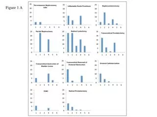
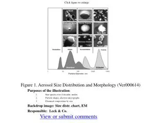
Figure 1. Particle size distribution of a bentonite suspension after four settlings. Figure 2. Influence of the time step t on the k -value determination by using the representation for the experiment using a 0.2 µm membrane ( C = 10 -2 g/L and P = 0.3 bar). Step III. Step II.

E N D
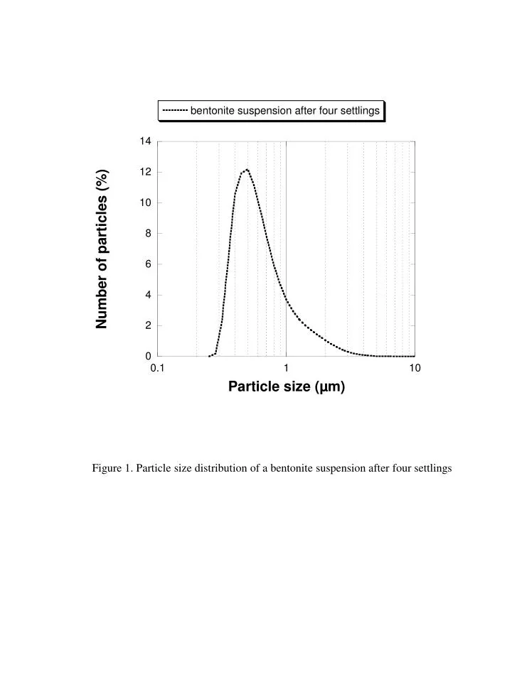
Figure 1. Particle size distribution of a bentonite suspension after four settlings
Figure 2. Influence of the time step t on the k-value determination by using the representation for the experiment using a 0.2 µm membrane (C = 10-2 g/L and P = 0.3 bar)
Step III Step II Step I n = 2 n > 2 n = 0 Figure 3. Example of the determination of the slope n in the representation for the fouling mechanisms identification ( experimental data for 5 µm membrane; C = 10-2 g/L and P = 0.3 bar)
(A) QB,0 (B) n =2 VB,0 (C) n = 0 VC,0 Figure 4. Split of the curves into successive mechanisms: (A) very low fouling mechanism , ( B) blocking , (C) cake filtration.
Figure 5. Plot of cumulative permeate volume V versus time t - comparison between experimental and calculated curves for four experiments (C = 10-2 g/L and P = 0.3 bar): ( 0.2 µm; 0.8 µm; 5 µm; 8 µm)
Figure 6. Effect of the transmembrane pressure P on the final surface coverage ratio, B,f for two different membranes (0.2 µm and 8 µm)
Figure 7. Symbols are the values of VB,f – VB,0 versus B, for a series of data (dpore = 0.2; 0.8; 5; 8 µm). Operating conditions were kept the same for all these experiments: C = 10-2 g.L-1, P = 0.3 bar. Lines are the calculated data of VB,f – VB,0 versus B, for different values of B,f
Figure 8. Evolution of a clean and fouled filter media resistance (respectively, Rm,0 and RmB,f) with its initial mean pore diameter, dpore
Figure 9. Effect of feed suspension concentration C on the specific parameter, C, for cake formation at constant pressure 0.3 bar
Figure 10. Effect of feed suspension concentration C on the specific parameter, B, for pore blockingat constant pressure 0.3 bar
Figure 11. Plot of B versus the product of feed concentration, C times the number of blocked pores per unit of blocking particle, p/pore (Cp/pore) at constant pressure 0.3 bar
Figure 12. Effect of transmembrane pressure on cake formation: comparison between two membranes (0.2 µm and 8 µm) by considering the plot of C /C1.1 versus P
Figure 13. Effect of transmembrane pressure on pore blocking for two different membranes (0.2 µm and 8 µm) by considering the plot of B versus P
Figure 14. Effect of the wall shear stress, w on pore blocking mechanism for two different membranes (0.2 µm and 8 µm)
Figure 15. Effect of the mean pore diameter of the filter media on the specific parameter, B, for pore blocking (C = 10-2 g/L and P = 0.3 bar)