Download
1 / 20
200 likes | 210 Views
Explore convective mass flows and heat transfer in reversible and irreversible thermodynamics. Understand fluid movement, wave equations, turbines, compressors, and heat exchanges in mass transport phenomena.

E N D
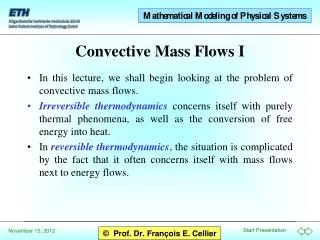
In this lecture, we shall begin looking at the problem of convective mass flows. Irreversible thermodynamics concerns itself with purely thermal phenomena, as well as the conversion of free energy into heat. In reversible thermodynamics, the situation is complicated by the fact that it often concerns itself with mass flows next to energy flows. Convective Mass Flows I
Mass flow vs. entropy flow Fluid moving through a pipe Wave equation Forced flow Turbines Compressors and pumps Heat flow Mass transport losses Table of Contents
Although there exist phenomena that take place purely in the thermal domain, there can be no mass flows that occur without heat flows accompanying them. The problem has to do with the fact that mass flows always carry their volume and stored heat with them. It is therefore not meaningful to consider these quantities independently of each other. The water circulation within Biosphere 2 may serve as an excellent example. The thermal phenomena of the water cycle cannot be properly described without taking into account its mass flow (or at least its volume flow) as well. Mass Flows vs. Entropy Flows
We shall start by modeling the flow of fluids (liquids or gases) in a pipe. The pipe can be subdivided into segments of length Dx. If more fluid enters a segment than leaves it, the pressure of the fluid in the segment must evidently grow. The fluid is being compressed. qin p C : 1/c p = c · ( qin – qout ) dp qout Dq dt Fluid Moving in a Pipe I
When the pressure at the entrance of a segment is higher that at the exit, the speed of the fluid must increase. This effect is caused by the mechanical nature of the fluid. The pressure is proportional to a force, and the volume is proportional to the mass. Consequently, this is an inductive phenomenon. It describes the inertia of the moving mass. = k · ( pin – pout ) dq dt Dp pin I : 1/k q q pout Fluid Moving in a Pipe II
Consequently, the following bond graph may be proposed: C C C C Dqi ... ... pi pi+1 0 0 1 1 0 1 0 qi-1 qi Dpi I I I Fluid Moving in a Pipe III
Although the hydraulic/pneumatic inductor describes the same physical phenomenon as the mechanical inductor, its measurement units are nevertheless different. dq dp dt dt m3 ·s-1 [C] = [Dq] / [dp/dt] = = m4·s2·kg-1 Dp = L · Dq = C · N·m-2·s-1 [L] = [Dp] / [dq/dt] = = kg·m-4 N·m-2 is still a time constant [ L·C ] = s m3 ·s-2 Capacitors and Inductors
Any text book of physics teaches us that moving fluid in a pipe satisfies the wave equation. Discretization in space leads to: 2p 2p = c 2· 2 t 2 x 2 ( ) Dx · c d2pk · ( pk+1 – 2 · pk + pk-1 ) = c 2 dt 2 Dx2 d2pk = pk+1 – 2 · pk + pk-1 dt 2 The Wave Equation I
The following replacement circuit comes to mind: L·C L L dvi /dt = iC /C iC = iL1 – iL2 vi-1 – vi = L· diL1 /dt vi – vi+1 = L· diL2 /dt iL1 iL2 iC C v v v v C·d2vi /dt2 = diC /dt diC /dt = diL1 /dt – diL2 /dt vi-1 – vi = L· diL1 /dt vi – vi+1 = L· diL2 /dt i+1 i 0 i-1 = 0 d2vi Dx c = (L · C) · = vi+1 – 2·vi + vi-1 dt2 The Wave Equation II
A chain of such links indeed corresponds to the proposed bond graph: L L L L C C C C C C C ... ... 0 0 0 0 1 1 1 I I I The Wave Equation III
A forced flow can first be conceptualized as a modulated flow source. Sf Sf q q ... ... C C C C q 0 0 0 0 1 1 I I The Forced Flow I What happens with the energy at the interrupted chain? As the flows to the left and to the right are identical (mass conservation), it makes sense to unite the two flow sources.
q p2 p1 Sf q q Se ... ... A flow cannot be forced without adding energy to the system. Unfortunately, there is a small problem: the energy conservation is violated! C C C C 0 0 0 0 1 1 I I The Forced Flow II It seems that we need to look at this problem a little more carefully ...
We shall check what happens, when the blade of a turbine is placed in the path of a flow that occurs for reasons external to the model. The pressure difference on the two sides of the blade generates a resulting force that produces a torque in the turbine. The generated torque is proportional to the pressure difference, and consequently, we recognize the effects of a bond-graphic transformer at work. If the turbine is designed optimally, the pressure difference is fully converted to a torque, i.e., no hydraulic energy is left to be stored in an inductor. The Turbine I
C C C C ... ... pi pi+1 0 1 0 1 0 qi qi 0 1 Dpi qi I TF w t I I:J 1 R:B The Turbine II The pressure difference pi leads to a torque . This in turn generates an angular velocity at the turbine, which induces a flow qi back on the hydraulic side.
Cause and effect can also be reversed. We can generate a torque at the turbine by means of a DC-motor sitting on the same axle. The turbine together with the motor is now called either compressor or pump. This device induces a flow qi on the hydraulic side, which causes a corresponding pressure difference. Compressors and Pumps I
C C C C water pipe 0 1 The DC-motor together with the pump replace the non-linear (modulated) flow source that had been postulated earlier. I DC-motor compressor / pump Compressors and Pumps II I ... ... pi pi+1 0 1 0 1 0 qi qi qi Dpi TF I:La w t ui tm u Se GY 1 1 R:B w R:Ra I:J
We have meanwhile understood, how the mass flow needs to be modeled. However, the transported mass always carries its own heat along. When modeling thermal phenomena, it is therefore important, to correctly represent these heat flows, which are not of a dissipative nature. q . . . = S V Heat flow S S S Storage V,S q Mass flow = (S/V) · q Heat Flow I
The resulting heat flow can indeed be represented as a non-linear (modulated) flow source. The energy conservation law is not violated here, since entropy is not conserved. ... Ti Ti+1 C C C . . 0 Sf Sf Sf 0 0 0 . Si Six Si 0 1 Cth Cth Cth Cth C S/V S/V S/V qi I ... ... pi pi+1 0 1 0 1 0 qi qi qi Dpi I TF Heat Flow II
Fluid transports are in reality always associated with losses due to friction. ... Ti Ti+1 C C C . . 0 Sf Sf Sf 0 0 0 . Six Si Si 0 1 Cth Cth Cth Cth C S/V S/V S/V RS RS RS qi I ... ... pi pi+1 0 1 0 1 0 qi qi qi Dpi I TF Mass Transport Losses
We have meanwhile understood that the cause ofconvective heat flows is to be found in the mass transport. The mass transport is captured by the wave equation, whereby forced flows (pumps, compressors) replace the inductors at the locations of flow-forcing devices. The heat flow is a consequence of the mass flow, and may be modeled using non-linear (modulated) internal flow sources. Frictional losses can be added to the model afterwards where and when needed. Conclusions