Download

1 / 45
500 likes | 682 Views
Explore methods like Newton-Raphson for finding square roots, zeros of functions, and system solutions. Includes examples and code snippets for implementation.

E N D
Root Finding The solution of nonlinear equations and systems Vageli Coutsias, UNM, Fall ‘02
The Newton-Raphson iteration for locating zeros
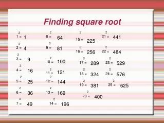
Example: finding the square root Details: initial iterate must be ‘close’ to solution for method to deliver its promise of quadratic convergence (thenumber of correct bits doublingwith every step)
Square root by Newton-Raphson % find square root of A x = (1+2*A)/3; maxiter = 20; for k = 1:maxiter x = (x+ (A/x))/2; end
functionx = sqrt1(A) if A < 0 break;end if A == 0; x = 0; else TwoPower = 1; m = A; while m >= 1, m = m/4; TwoPower = 2*TwoPower ;end while m < .25, m = m*4; TwoPower = TwoPower/2;end x = (1+2*m)/3; for k = 1:4 x = (x+ (m/x))/2; end x = x*TwoPower; end
function z = newton(func,z0,tol,maxiter,varargin) hopt = 2*sqrt(eps); z = z0; value = feval(func,z,varargin{:}); iter = 1; while abs(value) >=tol deriv = (feval(func,z+hopt,varargin{:}) - val)/hopt; z = z - value/deriv; value = feval(func,z,varargin{:}); iter = iter+1; if iter >= maxiter fprintf('maxiter exceeded, no convergence') break end end
function [z,varargout] = ... newton(func,z0,tol,maxiter,varargin) hopt = 2*sqrt(eps); z = z0; iter = 1 value = feval(func,z,varargin{:}); while abs(value) >=tol if iter >= maxiter fprintf('maxiter exceeded, no convergence'); break end deriv = (feval(func,z+hopt,varargin{:}) - val)/hopt; z = z - value/deriv; value = feval(func,z, varargin{:}); iter = iter+1; end ifnargout >= 2 ; varargout{1} = val; end ifnargout >= 3 ; varargout{2} = iter; end
functionzerofinder() clear; close all a=10; b = 3; x = linspace(-20,20,100); y = func(x,a,b); zz =zeros(100); plot(x,y,x,zz) [z,val,iter] = newton(@func,1,.0001,40,a,b) function z = func(y,a,b) z=y.^2+a*y+b; z = -0.30958376444732 val = 4.462736e-006 iter = 4
clc; close all; clear all; format long e; fname = 'func'; a = input('Enter a value:'); b = input('Enter b value:'); xc = input('Enter starting value:'); xmax = xc; xmin = xc; fc = feval(fname,xc,a,b); delta = .0001; fpc = (feval(fname,xc+delta,a,b)-fc)/delta; k=0;disp(sprintf('k x fval fpval ')) while input('Newton step? (0=no, 1=yes)') k=k+1; x(k) = xc; y(k) = fc; xnew = xc – fc / fpc; xc = xnew; fc = feval(fname,xc,a,b); fpc = (feval(fname,xc+delta,a,b)-fc)/delta; disp(sprintf('%2.0f %20.15f %20.15f %20.15f',k,xc,fc,fpc)) if xmax <= x(k); xmax = x(k); end if xmin >= x(k); xmin = x(k); end end x0 = linspace(xmin,xmax,201); y0 = feval(fname,x0,a,b); plot(x0,y0,'r-',x,y,'*')
Enter a value:.1 Enter b value:.5 Enter starting value:0 k x fval Newton step? (0=no, 1=yes)1 1 -0.454545455922915 0.028917256044793 2 -0.486015721951951 0.000349982958035 3 -0.486406070359515 0.000000068775315 4 -0.486406147091071 0.000000000002760 5 -0.486406147094150 0.000000000000000 Newton step? (0=no, 1=yes)0
function f = func(x,a,b) % trap near x = 0 % for interesting behavior, use a = .1, b = .0001, x0 = .4 f = .5*x.^2+ 100*x.^8 - a*x.^16 + b;
% script zeroin % uses matlab builtin rootfinder "FZERO" % to find a zero of a function 'fname' close all; clear all; format long %fname = 'func'; % user defined function-can also give as @func %fpname='dfunc'; % user def. derivative-not required by FZERO del = .0001;% function value limiting tolerance a = input('Enter a value:'); b = input('Enter b value:'); x0 = linspace(-10,10,201); y0 = feval(@func,x0,a,b); xc = input('Enter starting value:'); %root = fzero(@func,xc,.0001,1,a,b); % grandfathered format OPTIONS=optimset('MaxIter',100,'TolFun',del,'TolX',del^2); root = fzero(@func,xc,OPTIONS,a,b) y = feval(@func,root,a,b) plot(x0,y0,root,y,'r*')
The planar 4-bar linkage can assume various configurations. For each value of the angle f there are two possible values of y and vice versa. The mid-point of the bar CD executes a complex motion.
function linkage() close all; a1=10;a2=5;a3=7;a4=2; psi0=30; A=[0,0]; B=[a1,0]; axis equal for i = 1:60 phi(i)=i*pi/30; psi(i) = fzero(@bar4,psi0,[],phi(i),a1,a2,a3,a4); C=[a1+a2*cos(psi(i)),a2*sin(psi(i))]; D= [a4*cos(phi(i)),a4*sin(phi(i))]; XX=[A,B,C,D,A]; plot(XX(:,1),XX(:,2),'k-') hold on x = (a1+a2*cos(psi)+a4*cos(phi))/2; y = (a2*sin(psi)+a4*sin(phi))/2; plot(x,y,'ro'); pause(.1) plot(XX(:,1),XX(:,2), 'y-') end plot(XX(:,1),XX(:,2),'k-')
Application: solution of a BVP (Boundary Value Problem) Solution
Problem Solve previous equation for the smallest suitable nonzero value of k (eigenvalue) using (a) The Newton method (script ‘NEWT.M’) (b) The built-in Newton method (script ‘ZEROIN.M’) (c) The secant method (script ‘SEC.M’)
FIXED POINT ITERATIONS Unique fixed point in interval [a,b]
Error estimate use difference between successive iterates to estimate error
Newton iteration as fixed-point iteration: quadratic convergence
Example: the logistic map What happens if uniqueness is violated?
function fixed_point() close all a = .9; tol = 10^(-16); imax = 1000; i = 1; deltax = 1; x(1) = .01; while deltax >= tol & i <= imax x(i+1) = f1(x(i),a); deltax = abs(x(i+1)-x(i)); i = i+1; end n = length(x) xx = linspace(0,1,100); yy = f1(xx,a); plot(xx,xx,'g',xx,yy,'b',x(1:n-1),x(2,n),'ro') function y = f1(x,a) y = 4*a*x.*(1-x);
FMINBND Scalar bounded nonlinear function minimization. X = FMINBND(FUN,x1,x2) starts at X0 and finds a local minimizer X of the function FUN in the interval x1 < X < x2. FUN accepts scalar input X and returns a scalar function value F evaluated at X.
SPLINE Cubic spline data interpolation. YY = SPLINE(X,Y,XX) uses cubic spline interpolation to find YY, the values of the underlying function Y at the points in the vector XX. The vector X specifies the points at which the data Y is given. If Y is a matrix, then the data is taken to be vector-valued and interpolation is performed for each column of Y and YY will be length(XX)-by-size(Y,2). PP = SPLINE(X,Y) returns the piecewise polynomial form of the cubic spline interpolant for later use with PPVAL and the spline utility UNMKPP. Ordinarily, the not-a-knot end conditions are used. However, if Y contains two more values than X has entries, then the first and last value in Y are used as the endslopes for the cubic spline. Namely: f(X) = Y(:,2:end-1), df(min(X)) = Y(:,1), df(max(X)) = Y(:,end) Example: This generates a sine curve, then samples the spline over a finer mesh: x = 0:10; y = sin(x); xx = 0:.25:10; yy = spline(x,y,xx); plot(x,y,'o',xx,yy)
PPVAL Evaluate piecewise polynomial. V = PPVAL(PP,XX) returns the value at the points XX of the piecewise polynomial contained in PP, as constructed by SPLINE or the spline utility MKPP. V = PPVAL(XX,PP) is also acceptable, and of use in conjunction with FMINBND, FZERO, QUAD, and other function functions. Example: Compare the results of integrating the function cos and this spline: a = 0; b = 10; int1 = quad(@cos,a,b,[],[]); x = a : b; y = cos(x); pp = spline(x,y); int2 = quad(@ppval,a,b,[],[],pp); int1 provides the integral of the cosine function over the interval [a,b] while int2 provides the integral over the same interval of the piecewise polynomial pp which approximates the cosine function by interpolating the computed x,y values.
% script SEC.M: uses secant method to find zero of FUNC.M close all; clear all; clc; format long e fname = 'func'; a = input('Enter a:');b = input('Enter b:'); xc = input('Enter starting value:'); fc = feval(fname,xc,a,b); del = .0001; k=0; disp(sprintf('k x fval fpval ')) fpc = (feval(fname,xc+delta,a,b)-fc)/delta; while input('secant step? (0=no, 1=yes)') k=k+1; x(k) = xc; y(k) = fc; f_ = fc; xnew = xc - fc/fpc; x_ = xc; xc = xnew; fc = feval(fname,xc,a,b); fpc= (fc - f_)/(xc-x_); disp(sprintf('%2.0f %20.15f %20.15f %20.15f',k,xc,fc,fpc)) end if x(1) <= x(k); xa = floor(x(1)-.5); xb = ceil(x(k)+.5); else; xb = floor(x(1)-.5); xa = ceil(x(k)+.5); end x0=linspace(xa,xb,201);y0=feval(fname,x0,a,b);plot(x0,y0,x,y,'r*')