Download
1 / 88
880 likes | 987 Views
Niloy Ganguly Department of Computer Science & Engineering Indian Institute of Technology, Kharagpur Kharagpur 721302. Growth models of Bipartite Networks. Contents of the presentation. Introduction to Bipartite network (BNW) and BNW growth Why BNWs ? Classes of Growth Models

E N D
Niloy Ganguly Department of Computer Science & Engineering Indian Institute of Technology, Kharagpur Kharagpur 721302 Growth models of Bipartite Networks
Contents of the presentation • Introduction to Bipartite network (BNW) and BNW growth • Why BNWs ? • Classes of Growth Models • Sequential attachment growth model (SA) • Parallel attachment with replacement growth model (PAWR) • parallel attachment without replacement growth model (PAWOR) • One-mode Projection • Model verification • Conclusions and future works
Contents of the presentation • Introduction to Bipartite network (BNW) and BNW growth • Why BNWs ? • Classes of Growth Models • Sequential attachment growth model (SA) • Parallel attachment with replacement growth model (PAWR) • parallel attachment without replacement growth model (PAWOR) • One-mode Projection • Model verification • Conclusions and future works
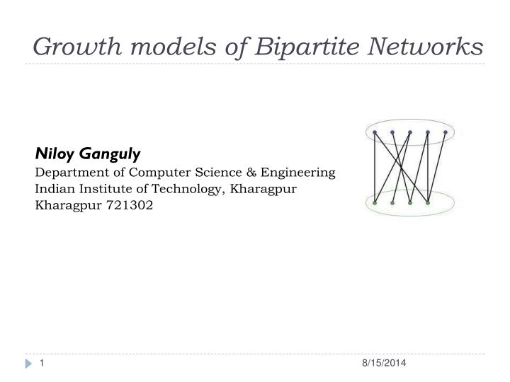
Bipartite network (BNW) • Two disjoint sets of nodes, namely “TOP” set and “BOTTOM” set • No edge between the co-members of the sets • Edges - interactions among the nodes of two sets Top Set Bottom Set
BNW growth • One top node is introduced at each time step • Top nodes enter the system with µ edges ( 1≤ µ) • Each top node can bring m new bottom nodes (1≤ m <µ). If m=0, the bottom set is fixed. • Edges are attached randomly or preferentially
Contents of the presentation • Introduction to Bipartite network (BNW) and BNW growth • Why BNWs ? • Classes of Growth Models • Sequential attachment growth model (SA) • Parallel attachment with replacement growth model (PAWR) • parallel attachment without replacement growth model (PAWOR) • One-mode Projection • Model verification • Conclusions and future works
Many real world examples • Many real systems can be abstracted as BNWs • Biological networks • Social networks • Technological networks • Linguistic Networks
A regulatory system network The output data are driven by regulatory signals through a bipartite network Liao J. C. et.al. PNAS 2003;100:15522-15527
Disease Genome Network Goh K. et.al. PNAS 2007;104:8685-8690
People Project Network Bipartite network of people and projects funded by the UK eScience initiatives The people are circles and the projects are squares. The color and size of the nodes indicates degree; redder and bigger nodes have more connections than smaller and yellower nodes
/θ/ L1 /ŋ/ L2 /m/ Languages Consonants /d/ L3 /s/ L4 /p/ Phoneme Language Network The Structure of the Phoneme-Language Networks (PlaNet)
And many others……. • Protein-protein complex network • Movie-actor network • Article-author network • Board-director network • City-people network • Word-sentence network • Bank-company network
Contents of the presentation • Introduction to Bipartite network (BNW) and BNW growth • Why BNWs ? • Classes of Growth Models • Sequential attachment growth model (SA) • Parallel attachment with replacement growth model (PAWR) • parallel attachment without replacement growth model (PAWOR) • One-mode Projection • Model verification • Conclusions and future works
Two broad categories • Both partitions grow with time • Empirical and analytical studies are available Ramasco J. J., Dorogovtsev S. N. and Pastor-Satorras R., Phys. Rev. E, 70 (036106) 2004. • Only one partition grows and other remains fixed • Couple of empirical studies but no analytical research
Two broad categories • Both partitions grow with time • Empirical and analytical studies are available Ramasco J. J., Dorogovtsev S. N. and Pastor-Satorras R., Phys. Rev. E, 70 (036106) 2004. • Only one partition grows and other remains fixed • Couple of empirical studies but no analytical research • with many real examples: Protein protein complex • network, Station train network, Phoneme language • network etc….
BNW growth with the set of bottom nodes fixed • Fixed number of bottom nodes (N) • One top node is introduced at each time step • Top nodes enter with µ edges • Edges get attached preferentially
Attachment Kernel • µ edges are going to get attached to the bottom nodes preferentially • Attachment of an edge depends on the current degree of a bottom node (k) (k + €) • γis the preferentiality parameter • Random attachment when γ= 0
Attachment Kernel • µ edges are going to get attached to the bottom nodes preferentially • Attachment of an edge depends on the current degree of a bottom node (k) Referred to as the attachment probability or the attachment kernel • γis the preferentiality parameter • Random attachment when γ= 0
Contents of the presentation • Introduction to Bipartite network (BNW) and BNW growth • Why BNWs ? • Classes of Growth Models • Sequential attachment growth model (SA) • Parallel attachment with replacement growth model (PAWR) • parallel attachment without replacement growth model (PAWOR) • One-mode Projection • Model verification • Conclusions and future works
Sequential attachment model • µ = 1 • Total number of edges = Total time (t) • Example: Language - Webpage
Bottom node degree distribution • Attachment probability : Notations: - # of bottom nodes - time or # of top nodes - preferentiality parameter - bottom node degree - degree probability distribution at time t • Markov chain model of the growth: • No asymptotic behavior – the degree continuously increases
Bottom node degree distribution • Attachment probability : Notations: - # of bottom nodes - time or # of top nodes - preferentiality parameter - bottom node degree - degree probability distribution at time t • Markov chain model of the growth: • Degree distribution function 23 8/15/2014
Approximated parallel attachment solution • Attachment probability : • Degree distribution function • Approaches to Beta– distribution f(x,α,β) for C =
Four regimes The four possible regimes of degree distributions depending on . (a) , (b) (c) (d)
Contents of the presentation • Introduction to Bipartite network (BNW) and BNW growth • Why BNWs ? • Classes of Growth Models • Sequential attachment growth model (SA) • Parallel attachment with replacement growth model (PAWR) • parallel attachment without replacement growth model (PAWOR) • One-mode Projection • Model verification • Conclusions and future works
Parallel attachment with replacement model (PAWR) • µ ≥ 1 • Total number of edges = µt • Example: Codon – Gene
Exact solution of PAWR • For random attachment, we can derive the attachment probability as Attachment probability of edges to a bottom node of degree k at time t
Exact solution of PAWR • For random attachment, we can derive the attachment probability as Attachment probability of edges to a bottom node of degree k at time t • Introducing preferentiality in the model
Exact solution of PAWR • Recurrence relation for bottom node degree distribution
Exactness of exact solution of PAWR Probability of having degree k Probability of having degree k Degree(k) Degree(k) • N = 20, t = 250, µ = 40, γ = 1 • γ = 16 Solid black curve –> Exact solution Symbols –> Simulation Dashed red curve –> Approximation Approximation fails but exact solution does well
Observations on PAWR • Degree distribution curve is not monotonically • decreasing for γ = 1 • Two maxima in bottom node degree distribution • plots
Observation - I Degree distribution curve is not monotonically decreasing for γ = 1 Probability of having degree k Degree(k) N = 50, µ = 50
Observation - I Degree distribution curve is not monotonically decreasing for γ = 1 Critical γ Probability of having degree k µ Critical γ vs. µ: N = 10 Degree(k) Critical γ – The value of γ for which distribution become monotonically decreasing with mode at zero N = 50, µ = 50
Contents of the presentation • Introduction to Bipartite network (BNW) and BNW growth • Why BNWs ? • Classes of Growth Models • Sequential attachment growth model (SA) • Parallel attachment with replacement growth model (PAWR) • parallel attachment without replacement growth model (PAWOR) • One-mode Projection • Model verification • Conclusions and future works
Parallel attachment without replacement (PAWOR) • µ≥ 1 • Total number of edges = µt • No parallel edge • Example: Language - Phoneme
PAWOR Model - I • µ edges connect one by one to µ distinct bottom nodes • After attachment of every edge attachment kernel changes as • Theoretical analysis is almost intractable W is the subset of bottom nodes already chosen by the current top node
Degree distribution for PAWOR Model - I Probability of having degree k Probability of having degree k Degree(k) Degree(k) • N = 20, t = 50, µ = 5, γ = 0.1 • γ = 3
Degree distribution for PAWOR Model - I Probability of having degree k Probability of having degree k Degree(k) Degree(k) • N = 20, t = 50, µ = 5, γ = 0.1 • γ = 3 Approximated solution is very close to Model-I
PAWOR Model - II • A subset of µ nodes is selected from N bottom nodes preferentially. NCμsets • Attachment of edges depends on the sum of degrees of member nodes • Each of the selected µ bottom nodes get attached through one edge with the top node
Attachment kernel for subset • Attachment kernel for µ member subset - time or # of top nodes - preferentiality parameter - A µ member subset of bottom nodes - degree of the ith member node
Attachment kernel for subset • Attachment kernel for µ member subset - time or # of top nodes - preferentiality parameter - A µ member subset of bottom nodes - degree of the ith member node We need attachment probability for individual bottom node
Attachment probability for a single node • Attachment probability for a bottom node is sum of the attachment probabilities of all container subsets • Any specific bottom node (b) is member of number of subsets • Among those subsets any other bottom node except b has membership in number of subsets • Sum of degrees of all nodes is
Attachment probability for a single node • Attachment probability for bottom nodes
Bottom node degree distribution • Markov chain model of the growth:
Degree distribution for PAWOR Model - II Probability of having degree k Probability of having degree k Degree(k) Degree(k) • N = 20, t = 50, µ = 5, γ = 0.1 • γ = 3 • dotted lines for approximated parallel attachment model
Degree distribution for PAWOR Model - II Probability of having degree k Probability of having degree k Degree(k) Degree(k) • N = 20, t = 50, µ = 5, γ = 0.1 • γ = 3 • dotted lines for approximated parallel attachment model Only skewed binomial distributions are observed Extra randomness in the model
Contents of the presentation 48 • Introduction to Bipartite network (BNW) and BNW growth • Why BNWs ? • Classes of Growth Models • Sequential attachment growth model (SA) • Parallel attachment with replacement growth model (PAWR) • parallel attachment without replacement growth model (PAWOR) • One-mode Projection • Model verification • Conclusions and future works 8/15/2014
One mode projection of bottom Goh K. et.al. PNAS 2007;104:8685-8690
Degree of the nodes in One-mode • Easy to calculate if each node v in growing partition enters with exactly (> 1) edges • Consider a node u in the non-growing partition having degree k • u is connected to k nodes in the growing partition and each of these k nodes are in turn connected to -1 other nodes in the non-growing partition • Hence degree q=k(-1)