Download
1 / 35
350 likes | 481 Views
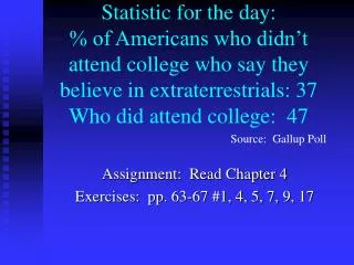
381. Statistic for the day: Number of words in English that exist because of typographical errors or misreadings:. Source: OED. Assignment: Read Chapter 15, pp 254-264 Exercises pp 271-275: 1, 2, 3, 9, 11, 12, 17.

E N D
381 Statistic for the day:Number of words in English that exist because of typographical errors or misreadings: Source: OED Assignment: Read Chapter 15, pp 254-264 Exercises pp 271-275: 1, 2, 3, 9, 11, 12, 17 These slides were created by Tom Hettmansperger and in some cases modified by David Hunter
Research question: Is ghost sighting related to age? Do young and old people differ in ghost sighting? The skeptic responds by saying he doesn’t believe that there is any difference between the age groups. We need to see the data to resolve the debate. Then we can consider assessing the risk. Exercise 9, p219 of the text.
Expected counts are printed below observed yes no Total young 212 1313 1525 174.9 1350.1 old 465 3913 4378 502.1 3875.9 Total 677 5226 5903 Chi-Sq = 7.870 + 1.020 + 2.742 + 0.355 = 11.987 The research advocate wins and skeptic loses. There is evidence in the data that there are differences in the population.
The percent of young who saw a ghost: 212/1525 = .139 Answer: 13.9% The proportion of old who saw a ghost: 465/4378 = .106 Answer: .106 The risk of young seeing ghost: Answer: 212/1525 or .139 or 13.9% Odds ratio?
Odds • The odds of something happening are given by a ratio: • For example, if you flip a fair coin, the odds of heads are 1 (or sometimes “1 to 1”). • An odds ratio is the ratio of two odds!
The odds that a young person saw a ghost: 212/1313 = .161 The odds that an older person saw a ghost: 465/3912 = .119 The odds ratio: Answer: .161/.106 = 1.35
Relative risk of young person seeing a ghost compared to older person: Answer: .139/.106 = 1.31 We would say that the risk that a younger person sees a ghost is 1.31 times higher than the risk that an older person sees a ghost. The increased risk that a young person sees a ghost over that of an older person: Answer: (.139 - .106)/.106 = .31 Hence we would say that young people have a 31% higher risk of seeing a ghost than older people.
Response: Calories Arby’s Explanatory: Size
Expected counts are printed below observed low high Total 1 5 2 7 3.50 3.50 2 2 5 7 3.50 3.50 Total 7 7 14 Chi-Sq = 0.643 + 0.643 + 0.643 + 0.643 = 2.571 Question: What happens if we had observed data 10 times bigger? So the skeptic wins.
Expected counts are printed below observed low high Total 1 50 20 70 35.00 35.00 2 20 50 70 35.00 35.00 Total 70 70 140 Chi-Sq = 6.429 + 6.429 + 6.429 + 6.429 = 25.714 Now the research advocate wins.
The point: sample size • Statistical significance is related to • the size of the sample. But that makes • sense. More data, more information, more • precise inference. • So statistical significance is related to two things: • The size of the difference between the percentages. • Big differences are more likely to show stat. significance. • 2. The size of the sample. Bigger samples are more likely • to show statistical significance irrespective of the size of • the difference in percentages.
Research question: Is ethnicity related to mortgage approval rates? approv not approv Total Af. Am. 3117 979 4096 76% White 71950 12997 84947 85% Total 75067 13976 89043 Chi-Sq = 32.714 +175.710 + 1.577 + 8.472 = 218.5 Research advocate wins big. (Exercise 19 p223 of the text.)
Notice that there were 89,043 applicants considered in the last example. The chi-squared value was 218.5. Suppose there were 100 times fewer, say about 890. Further, suppose the percentages of successful applicants were the same: 76% for African Americans and 85% for whites. Who do you think will win the debate, the research advocate or the skeptic? Why? The skeptic will win with a chi-squared value of 2.18.
Research question: Is there a relationship between whether you are sleep deprived and whether you typically smoke more than 0 packs per week? Rows: Sleepdep Columns: Smoke No Yes All No 96 23 119 80.67 19.33 100.00 Yes 86 26 112 76.79 23.21 100.00 All 182 49 231 78.79 21.21 100.00
Rows: Sleepdep Columns: Smoke No Yes All No 96 23 119 80.67 19.33 100.00 Yes 86 26 112 76.79 23.21 100.00 All 182 49 231 78.79 21.21 100.00 Skeptic wins big!! No evidence in the data to suggest a difference in the population. Chi-Square = 0.521
Note that 23.2% of the people who feel sleep deprived smoke but only 19.3% of the people who do not feel sleep deprived smoke. The skeptic wins and we conclude that the difference could easily have happened by chance. There is no practical difference between the two percentages anyway. Just a 3.9% difference.
What happens if we have 100 times the sample sizes? And suppose the percentages stay the same. Consider non-sleep-deprived students who say they smoke more than 0 packs per week: So instead of 23/119 = .193 or 19.3% We have 2300/11900 = .193 or 19.3% (same percent)
Rows: Sleepdep Columns: Smoke (Observed and expected counts shown) No Yes All No 9600 2300 11900 9375.76 2524.24 11900.00 Yes 8600 2600 11200 8824.24 2375.76 11200.00 All 18200 4900 23100 18200.00 4900.00 23100.00 Chi-Sq = 5.363 + 19.921 + 5.698 + 21.166 = 52.148 And now the research advocate wins and thedifference is statistically significant. But the difference of 3.9% is still not practically significant.
The point: practical significance Even if the difference in percentages is uninteresting and of no practical interest, the difference may be statistically significant because we have a large sample. Hence, in the interpretation of statistical significance, we must also address the issue of practical significance. In other words, you must answer the skeptic’s second question: WHO CARES?
Research question: Is the Salk polio vaccineeffective?Randomized experiment, double blindedCarried out in 1954 on 400,000 children.
Control proportion = 142/200,000 = .00071 or .071% Treatment proportion = 56/200,000 = .00028 or .028% Difference: Control – Treatment = .00043 or .043% Very small difference. But this was expected so they took large samples. But is the difference significant? Does the research advocate (Dr. Jonas Salk) win?
Expected counts are printed below observed polio not Total C 142 199,858 200,000 99 199,901 T 56 199,944 200,000 99 199,901 Total 198 399,802 400,000 Chi-Sq = 18.677 + 0.009 + 18.677 + 0.009 = 37.372 The research advocate wins easily. We say that the vaccine is statistically significant. But is it practically significant?
Recall the difference in proportions for Contol – Treatment = .00043 This represents the proportion of children saved from polio by the vaccine. Population of US in 2000: 286,196,812. Population of Children under age of 20: 82,997,075 Number of children saved from polio by the vaccine: 82,997,075 times .00043 35,688 That is certainly practically significant.
Goal: Combine ideas from Chapter 4 on surveys and polls with ideas from Chapter 12 on testing for statistical significance in contingency tables.
Gallup Poll: Has drug abuse ever been a causeof trouble in your family? Research question: Is there a significant difference between 2000 and 1999? Is 22% - 17% = 5% a real difference?
First recall the margin of error Suppose the polls were each based on 1200 people. What is the margin of error for the percents in the table? Margin of error = 1/(square root of 1200) = .03 or 3%.
Plan • First we will create a sample count table from the • original Gallup Poll percentages. • Then we will use the 4 step statistical inference process • to see if the differences are statistically significant. • 3. If the research advocate wins, we will consider • the differences in the Gallup Poll as reflecting real • differences in the populations (1999 and 2000). • We will then compute the relative and increased risks • associated with drug abuse troubles in families from 1999 • and 2000. This would indicate how big the differences are.
To resolve the debate between the research advocate and the skeptic we need to conduct a chi-squared test. Remember the skeptic says the 5% difference occurred by chance. There is really no difference in the populations. But we cannot conduct a chi-squared test on a table of percents. We need raw counts. The Gallup Poll generally tells you what the sample sizes were for the survey. If they do not, then we will use 1200 since they usually use between 1000 and 1500.
Table of counts Gallup Poll: Has drug abuse ever been a causeof trouble in your family?
Obs = 264 yes no Total 1 264 936 1200 234.00 966.00 2 204 996 1200 234.00 966.00 Total 468 1932 2400 Chi-Sq = 3.846 + 0.932 + 3.846 + 0.932 = 9.556
Conclusion Since chi-squared = 9.556, the research advocate wins. There is evidence in the data that there are real differences between the populations. That is, we have detected statistically (in the samples) that the increase (from 1999 to 2000) in people who say there has been drug abuse problems in their family is really in the populations. Next look at the relative risk and the increased risk of having drug troubles in a family from 1999 to 2000. That is, consider the practical significance.
1. The relative risk of drug abuse troubles in a family • (from 1999 to 2000) is: • .22/.17 = 1.29 • So the risk of drug troubles is 1.29 times higher in • 2000 than in 1999. • 2. The increased risk of drug abuse troubles in a family • (from 1999 to 2000) is: • (.22 - .17)/.17 = .29 • So there is a 29% higher risk in 2000 for drug troubles • in a family than in 1999.
Summary • 1. First we created a sample count table from the original • Gallup Poll percentages. • Then we used the 4 step statistical inference process • to see if the differences were statistically significant. • 3. The research advocate won ( chisquare = 9.556). So • we can now consider the differences in the Gallup Poll • as reflecting real differences in the populations (1999 and • 2000). • We finished by computing the relative and increased risks • associated with drug abuse troubles in families from 1999 • and 2000.