Download
1 / 61
620 likes | 631 Views
Markov Cluster A lgorithm. Outline. Introduction Important Concepts in MCL Algorithm MCL Algorithm The Features of MCL Algorithm Summary. Graph clustering. Decompose a network into subnetworks based on some topological properties Usually we look for dense subnetworks. Graph clustering.

E N D
Outline • Introduction • Important Concepts in MCL Algorithm • MCL Algorithm • The Features of MCL Algorithm • Summary
Graph clustering • Decompose a network into subnetworks based on some topological properties • Usually we look for dense subnetworks
Graph clustering Algorithms: • Exact: have proven solution quality and time complexity • Approximate: heuristics are used to make them efficient Example algorithms: • Highly connected subgraphs (HCS) • Restricted neighborhood search clustering (RNSC) • Molecular Complex Detection (MCODE) • Markov Cluster Algorithm (MCL)
Graph Clustering Intuition: High connected nodes could be in one cluster Low connected nodes could be in different clusters. Model: A random walk may start at any node Starting at node r, if a random walk will reach node t with high probability, then r and t should be clustered together.
Definitions and Representation An undirected graph and its adjacency matrix representation. An undirected graph and its adjacency list representation.
Theorem. Let M be the adjacency matrix for graph G. Then each (i, j) entry in M r is the number of paths of length r from vertex i to vertex j. Note: This is the standard power of m, not a Boolean product.
K-path • Graph power • The kth power of a graph G: a graph with the same set of vertices as G and an edge between two vertices iff there is a path of length at most k between them • The number of paths of length k between any two nodes can be calculated by raising adjacency matrix of G to the exponent k • Then, G’s kth power is defined as the graph whose adjacency matrix is given by the sum of the first k powers of the adjacency matrix:
K-Path Clustering G3 G G2
All-Pairs Shortest Paths • Given a weighted graph G(V,E,w), the all-pairs shortest paths problem is to find the shortest paths between all pairs of vertices vi, vj∈ V. • A number of algorithms are known for solving this problem.
All-Pairs Shortest Paths: Matrix-Multiplication Based Algorithm • Consider the multiplication of the weighted adjacency matrix with itself - except, in this case, we replace the multiplication operation in matrix multiplication by addition, and the addition operation by minimization. • Notice that the product of weighted adjacency matrix with itself returns a matrix that contains shortest paths of length 2 between any pair of nodes. • It follows from this argument that An contains all shortest paths.
Markov Clustering (MCL) Markov process The probability that a random will take an edge at node u only depends on u and the given edge. It does not depend on its previous route. This assumption simplifies the computation.
MCL Flow of network is used to approximate the partition There is an initial amount of flow injected into each node. At each step, a percentage of flow will goes from a node to its neighbors via the outgoing edges.
MCL Edge Weight Similarity between two nodes Considered as the bandwidth or connectivity. If an edge has higher weight than the other, then more flow will be flown over the edge. The amount of flow is proportional to the edge weight. If there is no edge weight, then we can assign the same weight to all edges.
Intuition of MCL Two natural clusters When the flow reaches the border points, it is likely to return back, than cross the border. A B
MCL When the flow reaches A, it has four possible outcomes. Three back into the cluster, one leak out. ¾ of flow will return, only ¼ leaks. Flow will accumulate in the center of a cluster (island). The border nodes will starve.
Introduction—MCL in General • Simualtion of Random Flow in graph • Two Operations: Expansionand Inflation • Intrinsicrelationship between MCL process result and cluster structure
Introduction-Cluster • Observation 1: • The number of Higher-Length paths in G is large for pairs of vertices lying in the same dense cluster • Small for pairs of vertices belonging to different clusters
Introduction-Cluster • Oberservation 2: • A Random Walk in G that visits a dense cluster will likely not leave the cluster until many of its vertices have been visited
Definitions • nxn Adjacency matrix A. • A(i,j) = weight on edge from i to j • If the graph is undirected A(i,j)=A(j,i), i.e. A is symmetric • nxn Transition matrix P. • P is row stochastic • P(i,j) = probability of stepping on node j from node i = A(i,j)/∑iA(i,j)
Flow Formulation • Flow: Transition probability from a node to another node. • Flow matrix: Matrix with the flows among all nodes; ith column represents flows out of ith node. Each column sums to 1. 1 2 3 Flow 0.5 0.5 Matrix 1 2 3 1 1 24
1 1 1 1/2 1 1 1 1/2 Definitions Adjacency matrix A Transition matrix P
1 1/2 1 1/2 What is a random walk t=0
1 1 1/2 1/2 1 1 1/2 1/2 What is a random walk t=1 t=0
1 1 1 1/2 1/2 1/2 1 1 1 1/2 1/2 1/2 What is a random walk t=1 t=0 t=2
1 1 1 1 1/2 1/2 1/2 1/2 1 1 1 1 1/2 1/2 1/2 1/2 What is a random walk t=1 t=0 t=2 t=3
Probability Distributions • xt(i) = probability that the surfer is at node i at time t • xt+1(i) = ∑j(Probability of being at node j)*Pr(j->i) =∑jxt(j)*P(j,i) • xt+1 = xtP= xt-1*P*P= xt-2*P*P*P = …=x0 Pt • What happens when the surfer keeps walking for a long time?
Motivation behind MCL • Measure or Sample any of these—high-length paths, random walks and deduce the cluster structure from the behavior of the samples quantities. • Cluster structure will show itself as a peaked distribution of the quantities • A lack of cluster structure will result in a flat distribution
Important Concepts about MCL • Markov Chain • Random Walk on Graph • Some Definitions in MCL
Markov Chain • A Random Process with Markov Property • Markov Property: given the present state, future states are independent of the past states • At each step the process may change its state from the current state to another state, or remain in the same state, according to a certain probability distribution.
Random Walk on Graph • A walker takes off on some arbitrary vertex • He successively visits new vertices by selecting arbitrarily one of outgoing edges • There is not much difference between random walk and finite Markov chain.
Some Definitions in MCL • Simple Graph • Simple graph is undirected graph in which every nonzero weight equals 1.
Some Definitions in MCL • Associated Matrix • The associated matrix of G, denoted MG ,is defined by setting the entry (MG)pq equal to w(vp,vq)
Some Definitions in MCL • Markov Matrix • The Markov matrix associated with a graph G is denoted by TG and is formally defined by letting its qth column be the qth column of M normalized
Explanation to Previous Example • The associate matrix and markov matrix is actually for matrix M+I • I denotes diagonal matrix with nonzero element equals 1 • Adding a loop to every vertex of the graph because for a walker it is possible that he will stay in the same place in his next step
Markov Cluster Algorithm • Find Higher-Length Path • Start Point: In associated matrix that the quantity (Mk)pq has a straightforward interpretation as the number of paths of length k between vp and vq
Example-Associate Matrix MG (MG+I)2
Conclusion • Flow is easier with dense regions than across sparse boundaries, • However, in the long run, this effect disappears. • Power of matrix can be used to find higher-length path but the effect will diminish as the flow goes on.
Inflation Operation • Idea: How can we change the distribution of transition probabilities such that prefered neighbours are further favoured and less popular neighbours are demoted. • MCL Solution: raise all the entries in a given column to a certain power greater than 1 (e.g. squaring) and rescaling the column to have the sum 1 again.