Download
1 / 54
542 likes | 888 Views
Design of Curves and Surfaces by Multi Objective Optimization. Rony Goldenthal Michel Bercovier School of Computer Science and Engineering The Hebrew University of Jerusalem. Introduction. This work is about curves and surfaces :

E N D
Design of Curves and Surfaces by Multi Objective Optimization Rony Goldenthal Michel Bercovier School of Computer Science and Engineering The Hebrew University of Jerusalem
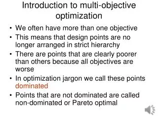
Introduction • This work is about curves and surfaces: • Fitting – finding surfaces (curves) as close as possible to a given set of points. • Design/Fairing – generate a surface achieving certain quality measures – design objective (minimal length, minimal curvature,…).
Introduction – cont. • Fitting alone is not sufficient, a certain quality of the resulting surface must be ensured. • Design alone is not sufficient, the surface must relate to some real world geometry – fitting is required. How to optimize several functions at once ?
Multiple Objective Functions • Suppose we want to incorporate several design objectives into a single optimization process: • Approximation error under L2 or Linf • Elastic energy • Length/Area • Class A criterions How to optimize several functions at once ?
Previous work • M. Alhanaty, M. Bercovier; R. Goldenthal, M. Bercovier: • Optimal Control in CAGD: • Decouple fitting from design • For each knot/parametrization configuration: • Solve the state equation (fitting) • Evaluate the cost function • Minimize the cost function (design objective)
Standard Approach :Weighted Sum of Objective Functions • Limitations: • Result depends on weights. • Some solutions cannot be reached. • Multiple runs of the algorithm are required in order to get the “whole picture”. • Difficult to select weights – cost functions may be in different scales.
ANSWER: Multi Objective Optimization • Multi objective solution does not have a single optimal solution, but an optimal solution set. • Possibility to implement a decision tool. • Natural set up for Genetic Algorithms.
Genetic algorithms for the single objective problem • The control variables: knot vector, parametrization and NURBS weights modeled as chromosomes. • Motivation for choosing single objective GA: • Highly non-linear behavior of knot vector modification • Support splines of any order (degree) • Support highly non linear cost functions • Support non-derivable cost functions • Elegant handling of constrains and singular conditions
Single Objective Genetic Algorithm (SOGA) - outline • [Start]Generate random population of n individuals. • [Fitness] Evaluate the f(x) of all x in the population. • [New population]Create a new population from the old population. • [Replace] the old population with the new one. • [Test] for end condition, stop, and return the best solution in current population. • [Loop] Go to step 2.
Single Objective Genetic Algorithm (SOGA) - outline • [Start] Generate random population of n individuals. • [Fitness] Evaluate the f(x) of all x in the population. • [New population]Create a new population by these steps (n times): • [Selection]Select two parents from the population according to their fitness. • [Crossover] performed with a crossover probability. • [Mutation] performed with a mutation probability. • [Accepting] Place new offspring in the new population. • [Replace] the old population with the new one. • [Test] for end condition, stop, and return the best solution in current population • [Loop] Go to step 2.
GA - Example • The parents: t0 = {0,0,0,0,0.14,0.29,0.43,0.57,0.71,0.86,1,1,1,1} t1 = {0,0,0,0,0.22,0.34,0.45,0.55,0.66,0.78,1,1,1,1} • Their encoding: et0 = {0.14,0.14,0.14,0.14,0.14,0.14,0.14} et1 = {0.22,0.12,0.11,0.10,0.11,0.12,0.22} • One Point crossover with split point = 4: ec0= {0.14,0.14,0.14,0.14,0.14,0.12,0.22} Normalization: ec0= {0.14,0.14,0.14,0.14,0.14,0.11,0.21}
GA – Example – cont. • Mutation: • Before: ec0 = {0.14,0.14,0.14,0.14,0.14,0.11,0.21} • After: ec0 = {0.14,0.13,0.13,0.15,0.14,0.11,0.21}
Multi Objective Genetic Algorithm • Multi objective optimization has an optimal solution set. • The main advantage of GA for MOO is that GA keeps a population and not a single solution. • The main difference between SOGA and MOGA is in the selection process.
MOGA - Selection • Better than and worse than relationships no longer hold. • Relationship among individuals is defined as “domination” relationship.
Domination • For any two solutions x1 and x2 x1 is said to dominate x2 if these conditions hold: • x1 is not worse than x2 in all objectives. • x1 is strictly betterthan x2 in at least one objective. • If one of the above conditions does not hold x1does not dominate x2.
Pareto Optimal Set • Non-dominated set: the set of all solutions which are not dominated by any other solution in the sampled search space. • Global Pareto optimal set: there exist no other solution in the entire search space which dominates any member of the set.
Multi Objective Genetic Algorithm – cont. • In each generation the non-dominated set is maintained, fitness is adjusted according to the domination of each individual. • In order to encourage diversity in the population fitness is reduced for similar solutions.
NURBS Curve • Input points: 28 • Control points: 20 • Order: 6 • Cost Functions: • L2 approximation error • Curve Length • Curvature
NURBS Curve Approximation Error: 1.12 Curve Length: 3.322 Curvature: 2,082
NURBS Curve Approximation Error: 0.36 Curve Length: 3.46 Curvature: 191.48
NURBS Curve Approximation Error: 0.075 Curve Length: 3.69 Curvature: 419.32
NURBS Curve Approximation Error: 0.0258 Curve Length: 3.707 Curvature: 2467.4
NURBS Surface I • Order: 4,4 • Input points: 8,8 • Control Points: 8,8 • Cost functions: • Surface Area • Surface Curvature
NURBS Surface Surface Area: 174 Surface Curvature: 4.9e-29
NURBS Surface Surface Area: 155.77 Surface Curvature: 0.099
NURBS Surface Surface Area: 155.16 Surface Curvature: 0.04
NURBS Surface Surface Area: 154.72 Surface Curvature: 0.12
NURBS Surface II • Order: 4,4 • Input points: 16,16 • Control Points: 5,5 • Cost functions: • Approximation Error • Surface Curvature
NURBS Surface Approximation Error: 5.807 Surface Curvature: 3.39
NURBS Surface Approximation Error: 5.19 Surface Curvature: 3.56
NURBS Surface Approximation Error: 2.46 Surface Curvature: 5.23
NURBS Surface Approximation Error: 1.348 Surface Curvature: 9.95
NURBS Surface Approximation Error: 1.256 Surface Curvature: 11.51
NURBS Surface Approximation Error: 0.937 Surface Curvature: 20.84
Summary • Decision tool for approximation and design. • Use of Multi Objective Genetic algorithm. • Result is a set of non-dominated solutions. • Implementation supports: NURBS curves and surfaces of arbitrary order. • Optimization variables: • Knot vector • Parameterization • NURBS weights
Summary • Support for various design objective: • Curves: • Length • Curvature • Approximation Error L2/Linf • Surfaces: • Curvature • Wilmore surfaces • Surface Area • Approximation error L2,Linf
Thank You! ronygold@cs.huji.ac.il http://www.cs.huji.ac.il/~ronygold
Applications • Surface fitting and design has numerous applications mainly in theses areas: • Industrial design. • Computer graphics. • Statistics.
Genetic Algorithms in CAD • Genetic algorithms in CAD, G. Renner and A. Ekárt • Data fitting with a spline using a real-coded genetic algorithm, F. Yoshimoto, T. Harada and Y. Yoshimoto • Genetic algorithms in free form curve design, A. Márkus, G. Renner and A.J. Váncza
GA - Encoding • Each individual contains 3 chromosomes: • One for Parametrization s. • One for Knot vector t. • One for the NURBS weights w. • Each chromosome is encoded by real valued numbers. • Intervals between two adjacent vector entries are actually stored (for s and t).
GA – Initial Population • The initial population was generated randomly while respecting validity constrains: • Positive NURBS weights. • Monotonically increasing parametrization and knot vector. • Sum of all intervals in parametrization and knot vector equals curve’s length. • Population size proportional to #(d.o.f).
GA – Fitness Evaluation • Interpolation/approximation must be performed prior to fitness evaluation. • For each individual in the population the fitness is evaluated. • Violation of Schoenberg-Whitney condition is penalized by the fitness evaluation.
GA - Crossover • Modified one point crossover used – for each chromosome with the following modification: • The sum of all the intervals that make the knot vector and the parametrization must remain fixed.
GA - Mutation • The mutation must respect these constrains: • All intervals must be positive. • Sum of all intervals must remain constant. • The mutation process (identical for all chromosomes): • Randomly select 2 intervals: i,j. • Randomly select x s.t. x < min(v(i),v(j)). • update: v(i) = v(i) + x; v(j) = v(j) – x;
GA - Selection • In SOGA selecting two parents is done is done randomly, when the probability of each individual to be a parent is proportional to its fitness. • Tournament, based on the above principle was used.
NURBS Curve Approximation Error: 1.08 Curve Length: 3.328 Curvature: 926.1