Download
1 / 17
170 likes | 179 Views
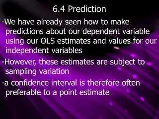
6.4 Prediction. -We have already seen how to make predictions about our dependent variable using our OLS estimates and values for our independent variables -However, these estimates are subject to sampling variation -a confidence interval is therefore often preferable to a point estimate.

E N D
6.4 Prediction -We have already seen how to make predictions about our dependent variable using our OLS estimates and values for our independent variables -However, these estimates are subject to sampling variation -a confidence interval is therefore often preferable to a point estimate
6.4 Prediction -Assume we want to obtain the value of y (denoted by θ) given certain independent values xj=cj: -since we don’t have actual values for BJ, our estimator of θ becomes:
6.4 Prediction -However, due to uncertainty, we may prefer a confidence interval estimate for θ: -Since we don’t know the above standard error, similar to F tests we construct a new regression using the calculation:
6.4 Prediction -substituting this calculation into the population regression function gives us: -In this regression, the intercept gives us the needed predicted value and intercept to construct our confidence interval -note that all our slope coefficients and their standard errors must be the same as the original regression
6.4 Prediction Notes 1) Note that the variance of this prediction will be smallest at the mean values of xj-This is due to the fact that we have most confidence in our OLS estimates in the middle of our data. 2) Note also that this confidence interval applies to the AVERAGE observation with the given x values, and does not apply to any PARTICULAR observation
6.4 Individual Prediction -When obtaining a confidence interval for an INDIVIDUAL (often one not in the sample), it is referred to as a PREDICITON INVERVAL and the actual outcome is: -x0 is the individual’s x values (which could be observed) and u0 is the unobserved error -Our best estimate of y0, from OLS, is:
6.4 Individual Prediction -given our OLS estimation, our PREDICITON ERROR is: -We know that E(Bjhat)xj=Bjxj (since OLS is unbiased) and E(u0)=0, therefore
6.4 Individual Prediction -Note that u0 is uncorrelated with Bjhat, since error comes from the population and OLS estimates are from a sample (and the actual error is uncorrelated with the estimated error) -Furthermore, u0 is uncorrelated with yhat0 -Therefore, the VARIANCE OF THE PREDICIOTN ERROR simplifies to:
6.4 Individual Prediction -The above variation comes from two sources: • Variation in yhat0. Since yhat0 comes from estimates of the Bj’s, which have a variance proportional to 1/n, Var(yhat0) is also proportional to 1/n, and is very small for large samples • σ2. Since (1) is often small, the variance of the error is often the dominant term
6.4 Individual Prediction -From our CLM assumptions, Bjhat and u0 are normally distributed, so ehat0 is also normally distributed. -Furthermore, we can rearrange our variance formulas to see that: -due to the σhat2 term, individual prediction CI’s are wider than average prediction CI’s and calculated as:
6.4 Residual Analysis -RESIDUAL ANALYSIS involves examining individual observations to determine whether the predicted value is above or below the true value -a negative residual can indicate an observation is undervalued or has an unmeasured characteristic that lowers the dependent variable -ie: a car with a negative residual is either a good deal or has something wrong with it (ie: it’s not a Ford)
6.4 Residual Analysis -a positive residual can indicate an observation is overvalued or has an unmeasured characteristic that increases the dependent variable -ie: a hockey team with a positive residual is either playing very well or has an unmeasured positive factor (ie: it’s from Edmonton, city of champions)
6.4 Predicting with Logs -It is very common to express the dependent variable of a regression using natural logs, producing the true and estimated equations: -Where xj can also be in log form -It may seem natural to predict y as: -But this UNDERESTIMATES yhat
6.4 Predicting with Logs -From our 6 CLM assumptions, it can be shown that: -Which gives us the simple prediction adjustment: -Which is consistent, but not unbiased, and depends highly on the error term having a normal distribution (MLR.6)
6.4 Predicting with Logs -Since in large samples normality isn’t required, forsaking MLR.6 we have -where α0=E(eu) -if we can estimate α0,
6.4 Predicting with Logs -In order to estimate α0hat, • Regress logy on all x’s and obtain logyhati’s: • For each observation, create mihat=elogyhati • Regress y on mihat without an intercept: 4) The coefficient on mihat is used to predict y
6.4 Comparing R2’s By definition, the R2 from the regression Is simply the squared correlation between the yi and the yihat. This can be compared to the square of the sample correlation for the regression In order to compare R2’s between a linear and log model.