Download
1 / 20
200 likes | 204 Views
This lecture discusses probability distributions, focusing on the normal distribution and its applications. It covers the central limit theorem, properties of the normal distribution, and how to calculate probabilities using Excel and MATLAB. Examples include the observed gravity over the UK and the Bouguer anomaly. The lecture also explores the impact of Icelandic volcanic ash on cloud formation and the use of percentiles in air quality directives.

E N D
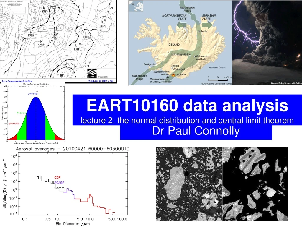
Dr Paul Connolly EART10160 data analysislecture 2: the normal distribution and central limit theorem
Week 8 practical – the normal distribution • What is a probability distribution? • The `normal distribution’ • How can we use them? • Distributions and percentiles. • The central limit theorem
Probability distribution • Basically it is a relative histogram with very small bin-widths • It describes how the data is distributed with regard to some property or variable. • This particular one is a normal distribution or `bell’-shaped curve
Histogram of observed gravity over the UK(log-normally distributed) • observed gravity over the UK is log-normally distributed. E.g. product of rock density; amount of rock below surface; etc. • Gravity (or density) anomalies are the sum of many variables => normally distributed. Positively skewed i.e. every so often it is higher than most of the values
The normal distribution is the most important distribution in statistics • Because many instruments have instrumental noise that results in a measurement being normally distributed (e.g. instrumental noise can be due to many factors). • Processes that depend on sum of many factors also tend to be normally distributed • Heights of people, IQ of people • Bouguer anomaly (effectively density of ground) • Freezing temperature of cloud drops (depends on what is in them). • Can easily use properties of normal distribution to apply to log-normally distributed data. But we will not use the lognormal distribution in this course
Frequency alone makes comparing the histograms difficult Dividing by the sum of the total and the bin width enables us to compare histograms What is probability density?(different histograms of data)
Properties of the normal distribution • Symmetrical about the mean • 99.9% of area within three standard deviations • 95.4% of area within two standard deviations • 68% within one standard dev.
Practise Qs • At exactly 0C a cheap digital thermometer has readings that are normally distributed with a mean of 0C and a standard deviation of 1 C. • What is the probability that the measurement reported is less than 0 C? • What is the probability that the measurement reported is greater than 0.5 C? • What is the probability that the measurement reported is between than -0.2 and 0.5 C? Excel use: NORMDIST(x,mean,std,1) MATLAB use: normcdf(x,mean,std);
The Bouguer anomaly • Difference between expected value of gravity and actual. • Tells you about how dense the underlying surface is. • For UK it is normally distributed.
More practise Qs • The Bouguer anomaly over the UK is normally distributed with a mean of -0.5 mGal and a standard deviation of 15 mGal • What is the fraction of UK area that has a Bouguer anomaly less than -0.5 mGal? • What is the fraction of UK area that has a Bouguer anomaly less than -15 mGal? (i.e. potential oil fields) • What is the fraction of UK area that has a Bouguer anomaly between -15 and 15 mGal? (i.e. no unknown oil fields or buried Meteorites) Excel use: NORMDIST(x,mean,std,1) MATLAB use: normcdf(x,mean,std);
Slides and data courtesy of Prof. G. Vaughan Impact of Icelandic volcano ashExpertise in the Centre for Atmospheric Science provided advice regarding the ash cloud of Icelandic volcanoes Centre for Atmospheric Science played leading role in the characterisation of volcanic ash during the Eyafyallajokull eruption in Iceland. Provision of advice to UK Government and Air Traffic agencies
LIDAR observations Clear skies meant that LIDAR observations could monitor the ash cloud • LIDAR measures backscattered light as a function of height and time. • Like a radar, using light rather than radio waves • Backscatter from air, clouds and aerosols as well as ash Scattering layer height time Pulse of light Light Detection And Ranging
First event: 15 April 2010 `Boundary Layer’ Note layers ~ 100 m thick. At Cardington they descend over time, being mixed into the BL Depolarisation plot shows that the particles are non-spherical=> ash. Hugo Ricketts, Univ. Manchester
Eyjafjallajökull volcanic ash impact on cloud formation • Ice `nucleation’ in supercooled water is a statistical effect. Freezing temperatures are normally distributed • Depends on fluctuations in water, which can be the sum of many things (heat, material diffusion, etc)
Percentiles • Value corresponding to location expressed as a percentage in a ranked list. • E.g. median is the 50th percentile. • Excel function PERCENTILE • MATLAB function prctile • Air quality directives from EU: • There should be no more than 18 exceedences of 200 micrograms per cubic metre for the hourly mean NO2 concentration in one year • Number of hours in 1 year: 365x24=8760 • Therefore if there are 18 exceedences then NO2 exceeds 200 g m-3 is for 18/(8760)=0.2055% of the time, or is less than 200 g m-3 for 100%-0.2055%=99.79% • So calculate the 99.79th percentile of the hourly means and if it is larger than 200 g m-3 there has been an exceedence
Using a smaller value for the percentile will underestimate the NO2 level. Data from a recent Public Inquiry(attention to detail)
Similar questions phrased a different way • The freezing temperature of drops containing volcano dust is normally distributed with a mean of -21C and a standard deviation of 1C • What temperature separates the upper 50% of drop freezing temps? i.e. the median. • What temperature separates the coldest 95% of freezing temperatures • Between what two temperatures are the 50% that are closest to the mean freezing temperature? i.e. the inter-quartile range. Take care with middle one! Excel use: NORMINV(P,mean,std) MATLAB use: norminv(P,mean,std);
Central limit theorem, page 10/11 notes • The distribution of sample means is a normal distribution with a standard deviation of the population standard deviation divided by sqrt(N). • E.g. if I select 1 drop at random from the population, with mean freezing temp -21C and standard deviation 1C, what is the probability its freezing temp will be less than -22C? • If I select a sample of 10 drops at random and calculate the mean freezing temperature what is the probability its freezing temp will be less than -22C?
/N0.5 Central limit theorem
Now • Same as last week – work through Practical PDF (check the notes if you are unsure of how functions work, etc) • Finish the Blackboard assessment in the week