Download

1 / 28
280 likes | 282 Views
Quarterly Economic Model. Nico van der Windt Marián Vávra Michal Andrle. Introduction. Joint development of the quarterly economic model (QEM) with SEOR, Erasmus Univ. Two parts of the project: Development of the core model Upgrade and refinement of the model

E N D
Quarterly Economic Model Nico van der Windt Marián Vávra Michal Andrle
Introduction • Joint development of the quarterly economic model (QEM) with SEOR, Erasmus Univ. • Two parts of the project: • Development of the core model • Upgrade and refinement of the model • The model is a story-telling device, with focus on medium term consistency of economic scenaria
Choice of the modelling paradigm (I) • Variety of possibilities to choose from • Capacity, time and technical constraints command compact structural model • The model is a structural keynesian model with neoclassical supply side • The model is built using top-down approach – emphasis put on joint and compact derivation of main behavioral relationships • Emphasis on long-run properties of the model
Choice of the modelling paradigm (II) Fitting data VAR’s Large-scale fully estimated Keynesian models Structural neoclassical top-down models (QEM) DSGE with solid microfoundations Theoretical rigor
Models Structural neoclassical models: • Euroarea-Wide Model (AWM), ECB • NiGEM (NIESR, UK) • JADE (CPB, NL) redesigned in 2003 • TRYM (Australian Treasury) • … and many others DSGE: • IMF’s GEM (Laxton, Pesenti et al.) Multicountry DSGE model,2004 • Bank of Canada QPM • Bank of England (BEQM) 2005 • October 2005 – Beneš, Hlédik, Kumhoff and Vávra: An Economy in Transition and DSGE: What the Czech National Bank’s New Projection Model Needs, CNB WP, Unpublished DRAFT
Treatment of expectations • Not much explicit treatment of the expectations • In the course of derivation of main behavioral eqs. adaptive expectations imposed • Idea – adjustment to new information is costly, partial adjustment used extensively • The model is fully backward-looking • We are not able to simulate expected shocks, etc • It is technically demanding to work with model-consistent expectations in medium-size nonlinear models. It also requires a lot of “tricks” (habit formation, ROT consumers…) to bring the model closer to stylized facts.
Estimation vs. Calibration • Earlier versions of the model mostly estimated with theoretical priors imposed • Current version mostly calibrated using all relevant information, strong reliance on theoretical priors • The model is not suited to capture short-term dynamics, but provides consistency needed in medium-term • ALL results are model-dependent and are subject to great uncertainty
Structure of the model (I) • Small Open Economy • Significant import intensity of exports • Sizeable ER pass-through • Elasticity of substitution between K and L lower than unity • Labor and goods market nominal and real rigidities • Markets do not clear in the model output-gap
Supply Side (I) • Aggregate good in the economy produced using domestic value added (GDP) and imported goods (total supply) • Domestic value added (GDP) formed by services of labor (L) and capital (K) • F(K,L) assumed CES with low elasticity of substitution (approx 1/3) F(GDP,M) K M F(K,L) L
Supply Side (II) • Demands for labour and capital are linked with the same price elasticity (elasticity of substitution) and unit income elasticity… -> consequence of using CES • Total factor productivity is exogenous exponential trend • Cost-per-unit of output derived as a theoretical counterpart to GDP deflator • Output gap is a part of the supply side • LR properties – Open-Economy Solow Model
Labour Market • Demand for labour derived together with demand for capital from the production function • Labour supply and population exogenous • Wage bargaining – “right-to-manage” approach to derive the wage equation • Reliance on theoretical priors
Investment and Capital Stock • Aggregate capital-stock in the economy enters the PF • Private investment derived from the firm’s profit optimization problem – demand for capital with large adjustment costs and investment/capital identity • Government nominal investment exogenous, entering PF and thus productive and capacity-enhancing • Initial (1993) government capital stock set approx 20 % of the total
Household sector • Consumption derived using RA model, assuming households view their wage income to follow random walk • Households are backward-looking in their decisions • Limited scope for wealth effects – empirical ambiguities, data problems…
Foreign Trade • Export demand driven by world trade and real exchange rate (demand approach) • Import demand driven by domestic demand, including exports, to account for the import intensity of exports (due to the supply side structure, where it is derived) • Price elasticity of exports twice as high as the one of imports • Current version does not distinguish goods and services
Price Block (I) • Price deflators derived as a theoretical counterparts to quantity variables • Cost-per-unit of output is the cost-of-living index from domestic value added PF. It is the weighted index of the price of labour and price of the capital. • Cost-per-unit of output is a counterpart to GDP deflator • Domestic/foreign content of the price indices calibrated. The domestic component consist of cost-per-unit of output, foreign component is the import deflator
Price Block (II) • Export deflator is derived under Semi-Small Open Economy Assumption, i.e. • The cycle-sensitive markup is represented by the output gap • The CPI is decomposed into administrative prices and core inflation, which is modeled. Overall CPI is then linked with consumption deflator • The existence of CPU allows us to treat GDP deflator as a residual variable, I.e. YP/Y
Fiscal Block (I) • Expenditures: • Government Investment (exog) • Government Wage Bill (LG exog, WG exog/rule) • Goods Consumption (exog in nominal terms) • Transfers and Benefits (UR Benefits, Pensions,…) • Interest rate payments • Incomes • Corporate and Personal Income Tax • VAT and excise tax • Social security contributions
Fiscal Block (II) • Disaggregated expenditure and revenue side allows us to assess the fiscal effects of economic shocks • Debt accumulation in the model moderately affects interest rates • Data issues: • The model has its own definitions not corresponding exactly to GFS or ESA… • Add-variables used to rescale the debt and deficit
Fiscal and Monetary Policy… • Monetary policy operates through simple IR rule (a la Taylor – inflation and output gaps sensitive) • What is the definition of the fiscal policy… ?? • Tax-rates and expenditures set.. Do we need more? • Is the “fiscal policy rule necessary” in the model…?? • Technically – NO, since expectations are not model-consistent and current response of the model is NOT affected by steady-state result and the model is solvable… • Economically – YES, • since permanent shocks let the debt explode/implode, which is even aggravated by interest response • Solvency of the government must be assured
Fiscal and Monetary Policy… • Fiscal policy then must be specified… • Intuitive and often questions: “What is the effect of increase in XY on … output, inflation… holding fiscal policy variables unchanged?” ARE problematic…
Example from using the model… • Variants of the model are used • 2003 – Pre-Accession Economic Program sensitivity analysis carried out using previous version of QEM World Trade Shock (Negative) Foreign Prices Shock
Example from using the model… • Since 2004 – more elaborated sensitivity analysis using scenaria is presented in the Convergence Program • Baseline, optimistic and pessimistic scenaria defined
Example from using the model… GDP (y-o-y, in %) Unemployment rate (in %) Current account (in % GDP) Public debt (in % GDP)
EX1: Government Consumption/Investment • What is the result of the same increase (in bill CZK) of • Government consumption? • Government investment? • Both are government expenditures… BUT investment is assumed to be productive and thus enhance the potential output of the economy… • Higher capacities lower the output gap and demand pressures, allowing for higher and more persistent growth of the economy. • The higher domestic prices, the lower exports and higher imports • Impact on unemployment… output effect vs. increase of real wages
EX1: Government Consumption/Investment GDP (scenario/baseline) GDP deflator Nominal Wages UR (p.b. from baseline)
EX2: Increase in World Demand • Assume permanent increase in foreign demand (level shift, not growth shift) • Exports reacts immediately… Import intensity of exports pulls imports upwards • Income effects also stimulates imports… Positive output gap slowly increase domestic prices… Having ER unchanged, changing RER shifts domestic demand to foreign goods • In the model, export prices are moderately affected by domestic prices, which have increased…
EX2: Increase in World Demand Imports and Exports response to the level shift in Y* (scenario/baseline)
EX2: Fiscal Rules Sensitivity • The model must contain fiscal rules, specifying the behaviour of the government • “No policy change” simulations are biased and/or inconsistent