“ Integrated Coastal Analyses” Demonstration Program in the Gulf of Mexico (REASoN)

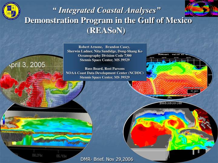
1. “ Integrated Coastal Analyses” Demonstration Program in the Gulf of Mexico (REASoN) Robert Arnone, Brandon Casey, Sherwin Ladner, Nita Sandidge, Dong-Shang Ko Oceanography Division Code 7300 Stennis Space Center, MS 39529 Russ Beard, Rost Parsons NOAA Coast Data Development Center (NCDDC) Stennis Space Center, MS 39529 DMR- Brief. Nov 29,2006

2. REASoN Objectives: • NASA supported for “bridging research and opreaions” for Coastal Applications • Establish environmental support products for the Gulf of Mexico • Demonstrate rapid access for monitoring ocean conditions • Automated data delivery and architecture for routine monitoring with ACT • Identify Metrics and product reliability and utility • Identify customers and applications through NASA and NOAA • Demonstrate real time monitoring of ocean conditions • Remote Sensing of bio-optical and thermal ocean properties • MODIS (AM, PM) • Modeling of the 3D ocean properties. NCOM/HYCOM • Identify new applications of ocean products for monitoring coastlines • New customized ocean products • Provide customized products using experimental monitoring • Identify Customers with NOAA / NASA – Target Focus areas • Harmful Algal Blooms • Fresh water Output - Hypoxia Creating and real time "Ocean Weather " capability

3. Reaching the Customers…. A Starting Architecture NASA Stennis MODIS Receive Site NRL Modeling Database NRL Remote Sensing Database SST Developmental Tools NRL Internal NRL External External Server Gulf of Mexico Revolving 30 Day real time NASA SSC Earth Science Applications Limited Access NOAA NOS Center for Coastal Monitoring and Assessment- DC NOAA NESDIS National Coastal Data Development Center -SSC ACT Server WIPE NOAA NOS / NCDDC Coastal Systems Center-Charleston NOAA NESDIS CoastWatch Program – DC Mississippi Dept. Of Marine Resources (DMR) Coastal Managers - Decision Makers

4. Products RRS – 412, 443,490,510,555,670 K532 Chlorophyll(OC3m, Carder) absorption (total, l) (A, C,QAA) aphi443 (Carder, OAA, Gould, Stumpf) adg412 (Carder, QAA, Stumpf) adg443(Carder, QAA,)ad412 (Gould) acdom (Gould) bb555(Arnone, Carder, QAA) Turbidity C648 (Gould) c670 (Carder) Horizontal Vis (QAA, Arnone) Vertical Vis (QAA, Arnone) Particulate Organic matter Particulate Inorganic Matter (Gould) Total Sus Sed (Gould) Water Mass (Gould) Cloud Albedo L2 Flags True Color Salinity 250M – True Color c670 (G&A) SST PAR Products - salinity, temperature, density - velocity (u,v), Sea Surface Height Dong Ko et al • Assimilation • Altimetry SSH • SST – (9 km) (MODIS 1km) • Synthetic BT (MODAS) • Forced by COAMPS • Resolution 6 km • 41 hybrid sigma/z levels • River fluxes (non-real time) • Driven by wind fields and heat fluxes Two Sets of real-time Monitoring Products Satellite products : Time MODIS – Terra –SST /Ocean Color MODIS – Aqua – SST /Ocean Color 2 scenes / day Circualation products : Physical Ocean Models – Navy Coastal Ocean Models (NCOM) - Nowcast – 12, 24 ,48 hour forecast Daily Products Total Satellite – 426 Model - 800 1226

5. MODIS Terra / Aqua, and SeaWIFS* Near Real-Time (2-4 hours) Level 3 Calibrated, Atmospheric Correction, Geophysical Product Geo-registered, daily composites 1 km resolution Level 4 Latest Pixel Composite Weekly, Monthly 1 km Level 4 Latest Pixel Composite Blend 1 2 3 4 5 6 7 SeaWIFS* 1 2 3 4 5 6 7 MODIS Terra 1 2 3 4 5 6 7 Daily product of the Latest Pixels New products Anomaly Salinity 3d- chlorophyll PAR Water Mass MODISAqua • Chlorophyll • atotal 443 • adg • bb555 • aphi • sst day • sst night * Not distributed (R&D Assessment)

6. CDOM Chlorophyll True Color Total Suspended Sediments Examples of Daily MODIS 1KM Products November 22, 2006

7. Coastal Applications Improved MODIS – 250m products Location of “turbid water” fronts  Fisheries and Oyster reef management Ship sampling – management Colored Water discharge Tidal Rips Tidal Rips through Channel Turbid Water Patches River Plume Winds streaks On coastal turbidity plumes 250m MODIS – Terra – Nov 14, 2004 Rayleigh corrected and Edge sharpening

8. MODIS 250 with the Tidal Currents Tuesday 24 Oct 2006 Next day changes in water quality !! Beyond a “Color Picture”  Quantitative “water” quality – “turbidity “ MODIS 250 with the Tidal Currents Monday 23 Oct 2006 Beam Attenuation Coefficient New capability for water quality management

9. April 3, 2005 0.05 0.11 0.26 0.58 1.3 March 12 March 23 March 10 MODIS – 250m products Monitoring Coastal processes PC-TIDES Beam Attenuation Coefficient

10. (-) Overestimated By Satellite (-) Underestimated By Satellite Salinity (PSU) J FM A MJ J A S O N D (Ladner et al. 2006 – Ocean Science) 10 15 20 25 30 35 Using Ocean Color Imagery to Monitor Salinity • Developed new ocean color algorithms • for retrieving surface salinity in coastal areas • - Defines extent of river plumes and coastal • runoff <10 (A) (B) 30 Error –Statistics 20 34 25 J FM A MJ J A S O N D

11. Seasonal Trends in Satellite Derived Salinity Fall Winter 2003 Spring Summer Salinity (PSU) 15 19 23 27 31 35

12. Coastal Modeling Forecasting Intra-Americas Sea Nowcast/Forecast System (c) (a) (d) (e) (f) (b)

13. NRL NCOM Model Characteristics • IAS NCOM Model • Resolution 6 km • 41 hybrid sigma/z levels • Data assimilating • Driven by wind fields and heat fluxes • Products • Temperature, salinity, currents, sea surface height • 48 hour forecast

14. Fusing the Satellite Optical Products and Physical Models Salinity SSH– NCOM SeaWIFS, MODIS Chlorophyll Absorption, Scattering, Photic Depth etc Currents – NCOM “Intra Americas Seas” • Naval Coastal Ocean Model (NCOM) • 41 Vertical layers, • Wind Forcing (CAMPS) • Assimilation of Altimetry and SST (MODIS) • River inputs Climatology • -Surface View Only

15. Real- Time Fusing of Remote Sensing With Ocean Models • Defines mesoscale features • model validation / verification • Provide user real time estimate of • quality of model / satellite products Sea Surface Temperature

16. Changing response of Physical and Bio-optical properties -Improved Understanding of Imagery Movement of Eddy Onshore Coastal Exchange Processes (mg/m3) .01 .054 .29 1.6 8.4 45.0 • Chlorophyll • Surface Currents • Sea Surface Height • Salinity Contour Cyclonic Eddy Mississippi River Plume Loop Warm core eddy Real time daily products New development of Subsurface Conditions

17. Mixed Layer Depth (m) 1/k –Satellite Penetration Depth Photic Depth Deriving the subsurface structure beyond the satellite observations Surface Chlorophyll Extended vertically Chl max

18. May 4 Subsurface Chlorophyll Properties by combining Satellites And Models Shelf 3d chlorophyll Going real time - Summer 2006 Photic Depth Movie May 4 Movie May 6

19. Forecasting Satellite Imagery / Optics Compare with MODIS March 2, 3, 2006 Seed the Model with Particles from MODIS March 1, 2006, Advect the particles forward Hourly steps Conservative tracers 24 hour forecast 48 hour forecast March 1, 2005 Backscatter Seed March 2, 2006 March 3, 2006 Seed Locations Observed Observed Original Seed Fields

20. March 1, advection- from currents 24 hours to March 2 Monitoring Coastal process Coupling Ocean Models with MODIS satellite products Plume dispersal Hourly changes in the coastal processes Backscattering “particle concentration”

21. Harmful Algal Bloom (HAB) Monitoring Targeting - Possible HARMFUL from non-HARMFUL ALGAL Supporting Ship Sampling regions measurement programs Assessing Size, Location and Movement of “Bloom” MODIS PRODUCTS Daily Potential HABS NO Anomaly Improved Decision Aide for Ship Sampling Sites Chlorophyll Oct. 9, 2005 62 day Mean YES Daily Real-Time Monitoring Advanced MODIS Bio-Optical Anomaly Products Under Evaluation Backscattering Next Day Forecast (Future Capability) CDOM detritus absorption

22. Data Transferred to NCDDC

23. 5 Real Time Daily updates Data Transferred to NCDDC

24. Changing Conditions MODIS Products used in Real-Time Coastal Observing Systems Fusing MODIS Products With Physical Models Ocean Atmosphere Providing Initialization Validation Defining Biological Response Monitoring the Coastal Response Providing Forecast and Prediction

25. Data Availability Models and Remote Sensing “Internal Browse” Of ongoing Products Outside Data available ftp Blended Products  NCDDC DODS interface . Data Fusion provides New capability http://colbalt.nrlssc.navy.mil:8000

26. Possibilities for NRL support to DMR? • Implementation of Decision Aids using Satellite • and Model Products • Automated product generation • Daily product delivery • Examples of Fecal Coliform algorithms from Chigbu, et al., 2005 • Time Series Data over Oyster Beds • Tracking dispersion of particles (or water masses) ????

27. Small boat oyster fisherman returning to Pass Christian Potential Applications of Oyster Reef Management in the Mississippi Sound Mississippi Department of Marine Resources / NOAA/Naval Research Laboratory High Turbidity MODIS Products Used for Managing Coastal Resources Solar Radiation (PAR) Decision Support MODEL Oyster Reef Closure Low SST • High levels of fecal coliform can contaminate or indicate contaminated oysters requiring DMR officials to close the oyster reefs • Fecal coliform die-off rates and predictions of concentration can be correlated to relative solar radiation, cloud cover, SST, river runoff (turbidity) and salinity. • NRL Stennis is providing MODIS derived estimates of solar radiation, SST, and turbidity as well as salinity estimates • NOAA NCDDC provides these data to Mississippi DMR for use in their fecal coliform decision tools. Low Salinity

28. Locating Turbidity fronts in the Mississippi Sound • Estuarine-dependent and coastal fish species production is enhanced in the vicinity of riverine discharges • Larval fish densities are highest at the associated turbidity fronts • Tracking overall turbidity in Mississippi Sound is important for monitoring the health of submerged aquatic vegetation (SAV) such as sea grasses • Large areas (some estimates as much as 60% of the total area) of SAV have been lost in Mississippi Sound in the past 30 years • SAV provides critical habitat for many recreational and commercial fish species • Sediment fall-out areas can be monitored for changing patterns of deposition and possible impacts from trawling and dumping of dredge spoils NRL 250 m MODIS derived turbidity in Mississippi Sound October 9, 2005 School of fish on clear side of turbidity front in Mississippi Sound

29. 8 Area IIA Cond. Approved Area IID Cond Approved 1 Area III Cond. Approved 7 2 Area IV Approved Area IIC Cond. Approved 6 Area IIB Approved Area IV Cond. Approved 9 Area IB Approved 5 Area II Approved 4 3 Area IV Approved Oyster Growing Areas in Mississippi Sound Tonguing Line Oyster Reefs Cond./Approved Oyster Growing Zones Prohibited Restricted Unclassified

30. Algorithms (1,4) Contain Salinity, Temp, River Stage Reef Location = 6 FC > 50 6 Fecal Coliform Estimates From Remote Sensing (Time Series Oct.28-Nov.18, 2006) Real-Time Implementation of Algorithms November 17, 2006 How does the FC Algorithms behave over Reef #6 for a 2 month period ? Fecal Coliform 15 17 19 21 23 25 • Relationships: • Log (FC) = 1.39 + 0.59(river stage) + 0.06(salinity) – 2.04Log(sst) • Log (FC) = 5.21 – 3.41Log(sst) • Log (FC) = -0.56 + 0.49(river stage) • Log (FC) = -0.99 + 0.72(river stage) – 0.04(sst) + 0.07(salinity) • Log (FC) = -0.40 + 0.43(river stage) • Log (FC) = 0.86 + 0.29(river stage) – 0.04(sst) Reference: Paulinus Chigbu, Scott Gordon and Paul B. Tchounwou. The Seasonality of Fecal Coliform Bacteria Pollution and its Influence on Closures of Shellfish Harvesting Areas in Mississippi Sound. International Journal of Environmental Research and Public Health. 2005. pp.362-373.

31. November 17, 2006 Fecal Coliform Levels Low -> High Based on threshold levels A “Warning” Image Can be created In Real-Time! November 17, 2006 Fecal Coliform Estimates Equation #6 High Levels Caution Low Levels Fecal Coliform Levels Derived From Remote Sensing Products 1 Km Log (FC) = 0.86 + 0.29(river stage) – 0.04(sst)

32. FC SUM PAR SUM PAR Fecal Coliform From Remote Sensing Time Series Reef #6 Product Comparisons Fecal Coliform vs. PAR OCT. 28 NOV. 09 Real-Time display of Remote sensing products At desired locations >15 FC <3.6 6 6 Inverse Relationship 6 6 Log (FC) = 0.86 + 0.29(river stage) – 0.04(sst)

33. FC FC TSS TSS Fecal Coliform From Remote Sensing (Eq.6) Time Series Product Comparisons Fecal Coliform vs. TSS OCT. 28 NOV. 09 >15 <3.6 6 6 Lag 6 6 Log (FC) = 0.86 + 0.29(river stage) – 0.04(sst)

34. Contamination Source Points (Continuous Seed) dispersed over 48 hours

35. Using a Dispersion Model, how does water disperse over the Oyster Reefs. ( 48 hours) Model Boundary

36. Summary – Ocean Weather • Real time ocean products are available through NRL – NCDDC (Unique capability to Mississippi and Gulf of Mexico ) • Presently we are establishing a model for U.S. Ocean Observing Systems • Establishing a “Ocean Weather” capability • NASA/NOAA/NRL working to provide a link of research to operations • Customized products are “easy” to develop from present architecture (See us) • Potential products are available to support “decision making process” • Ship sampling programs * Algorithm Implimentation • Potential “threat” areas • Historical studies / • Website / real time monitoring network exist at Stennis • Invitation to Visit real time room. • New Products are being generated monthly  GOOGLE EARTH • Request feedback on products and how products are used.

37. FC FC SALINITY SALINITY Fecal Coliform From Remote Sensing (Eq.6) Time Series Product Comparisons Fecal Coliform vs. Salinity OCT. 28 NOV. 09 >15 <3.6 6 6 Similar 6 6

38. FC FC SST SST Fecal Coliform From Remote Sensing (Eq.6) Time Series Product Comparisons Fecal Coliform vs. SST OCT. 28 NOV. 09 >15 <3.6 6 6 Similar 6 6

39. Oct. 13 – 19, 2004 Chl-a (mg/m3) .01 .054 .29 1.6 8.4 45.0 Latency (Days) Oct. 13 – 19, 2004 1 2 3 4 5 6 7 Level 4 Latest Pixel Composite Oct. 13, 2004 Oct. 14, 2004 Oct. 19, 2004 MODIS PM 7-Day For Chlorophyll-a (mg/m3) MODIS PM 7-Day For Latency / Pixel Age (Days) Oct. 15, 2004 Oct. 16, 2004 Oct. 17, 2004 Oct. 18, 2004

40. Chl-a (mg/m3) .01 .054 .29 1.6 8.4 45.0 Blending the “Latest Pixel Composite” from each satellite each day Terra September, 19 2004 Daily Bended Aqua

41. New Salinity products: Using Ocean Color Imagery to Monitor Salinity in the Northern Gulf of Mexico (-) Overestimated By Satellite (-) Underestimated By Satellite J FM A MJ J A S O N D Mississippi Bight 287 Stations Fort Lauderdale,FL 18 Stations Corpus Christi, TX 4 Stations Tampa Bay, FL 68 Stations Locations of Station Data used in Salinity Algorithm Development Chesapeake Bay, VA 108 Stations (A) (B) • For Barataria Bay Buoy, the derived salinities are estimated within 6 PSU’s between February and November and up to 15 PSU’s for December and January. • The satellite derived values are underestimated in the fall and winter months and over-estimated the majority of the time in the spring and summer. J FM A MJ J A S O N D (Ladner et al. 2006 – Ocean Science)

42. Daily Salinity Map Derived from Absorption Field Dec. 18, 2003 <10 20 30 34 20 25 Salinity (PSU) 10 15 20 25 30 35 Note: Low salinity waters are trapped off the coast of Louisiana near Barataria Bay and the Atchafalaya Basin. Major Fresh Water outflows occur during the winter months.

43. 250m Beam Attenuation Coefficient ( c ) TURBIDITY 250m True Color Examples of Daily MODIS 250m Products November 22, 2006

44. Current- nowcast, 24 , 48 hour forcast over the total absorption What causes the changes in currents? Winds?

45. Additional Anomaly fields Under evaluation for HABS targeting BB551 Backscattering Particle AT443 Absorption MODIS - Aqua Nov. 07, 2005 CHLOPHYLL Anomaly • New • Capability • ------------- • Anomaly • Fields • Scattering • Absorption • CDOM ADG412 Detrital and CDOM Absorption The absorption to scattering ratio (Single Scattering Omega) is linked to species identification. Requires evaluation with Cell Counts (with R. Stumpf). Present Chlorophyll Anomaly Product Products available in OPEN DAP.