Download
1 / 24
240 likes | 249 Views
Pfeifer note: Section 6. Class 26. Model Building Philosophy. Assignment 26. 1. T-test 2-sample ≡ regression with dummy T= +/- 6.2/2.4483 (from data analysis, complicated formula, OR regression with dummy) 2. ANOVA single factor ≡ regression with p-1 dummies (see next slide)

E N D
Pfeifer note: Section 6 Class 26 Model Building Philosophy
Assignment 26 • 1. T-test 2-sample ≡ regression with dummy T= +/- 6.2/2.4483 (from data analysis, complicated formula, OR regression with dummy) • 2. ANOVA single factor ≡ regression with p-1 dummies (see next slide) • 3. Better predictor? The one with lower regression standard error (or higher adj R2) • Not the one with the higher coefficient. • 4. Will they charge less than $4,500? • Use regression’s standard error and t.dist to calculate the probability.
Ready for ANOVA Ready for Regression
Agenda • IQ demonstration • What you can do with lots of data • What you should do with not much data • Practice using the Oakland As case
Remember the Coal Pile! • Model Building involves more than just selecting which of the available X’s to include in the model. • See section 9 of the Pfeifer note to learn about transforming X’s. • We won’t do much in this regard…
With lots of data (big data?) Stats like “std error” and adj R-square only measure FIT 2. Use the training set to build several models. Performance on a hold-out sample measures how well each model will FORECAST 1. Split the data into two sets 3. Use the hold-out sample to test/compare the models. Use the best performing model.
With lots of data (big data?) • Computer Algorithms do a very good job of finding a model • They guard against “over-fitting” • Once you own the software, they are fast and cheap • They won’t claim, however, to do better than a professional model builder • Remember the coal pile!
Without much Data • You will not be able to use a training set/hold out sample • You get “one shot” to find a GOOD model • Regression and all its statistics can tell you which model “FIT” the data the best. • Regression and all its statistics CANNOT tell you which model will perform (forecast) the best. • Not to mention….regression has no clue about what causes what…..
Remember….. • The model that does a spectacular job of fitting the past….will do worse at predicting the future than a simpler model that more accurately captures the way the world works. • Better fit leads to poorer forecasts! • Instead of forecasting 100 for the next IQ, the over-fit model will sometimes predict 110 and other times predict 90!
Requiring low-p-values for all coefficients does not protect against over-fitting. • If there are 100 X’s that are of NO help in predicting Y, • We expect 5 of them will be statistically significant. • And we’ll want to use all 5 to predict the future. • And the model will be over-fit • We won’t know it, perhaps • Our predictions will be WORSE as a result.
Modeling Balancing Act • Useable (do we know the X’s?) • Simple • Make Sense • Use your judgment, given you can’t solely rely on the stats/data • Signs of coefficients should make sense • Significant (low p) coefficients • Except for sets of dummies • Low standard error • Consistent with high adjusted R-square • Meets all four assumptions • Linearity (most important) • Homoskedasticity (equal variance) • Independence • Normality (least important)
Case Facts • Despite making only $40K, pitcher Mark Nobel had a great year for Oakland in 1980. • Second in the league for era (2.53), complete games (24), innings (284-1/3), and strikeouts (180) • Gold glove winner (best fielding pitcher) • Second in CY YOUNG award voting.
Nobel Wants a Raise • “I’m not saying anything against Rick Langford or Matt Keough (fellow As pitchers)…but I filled the stadium last year against Tommy John (star pitcher for the Yankees)” • Nobel’s Agent argued • Avg. home attendance for Nobel’s 16 starts was 12,663.6 • Avg. home attendance for remaining home games was only 10,859.4 • Nobel should get “paid” for the difference • 1,804.2 extra tickets per start.
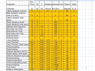
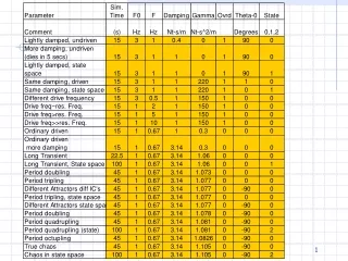
TASK • Be ready to report about the model assigned to your table (1 to 7) • What is the model? (succinct) • Critique it (succinctly) • Ignore “durban watson” • “standard deviation of residuals” aka regression’s standard error. • Output gives just t-stat. A t of +- 2 corresponds to p-value of 0.05.
What does it mean that the coefficient of NOBEL in negative in most of the models? Why was the coefficient of NOBEL positive in model 1?