Download
1 / 55
550 likes | 714 Views
Photon Position. Margaret Hawton, Lakehead University Thunder Bay, Canada. It has long been claimed that there is no photon position operator with commuting components and, as a consequence, no basis of localized states and no position space wave function, just fields and energy density.

E N D
Photon Position Margaret Hawton, Lakehead University Thunder Bay, Canada
It has long been claimed that there is no photon position operator with commuting components and, as a consequence, no basis of localized states and no position space wave function, just fields and energy density. In this talk I will argue that all of these limitations can be overcome! This conclusion is supported by our position operator publications starting in 1999.
Localizability The literature starts before 1930 and is sometimes confusing, in part because there are really 3 problems: • For any quantum particle ψ~e-iwtwith +ve w= and localizability is limited by FT theorems. • If all k's are equally weighted to localize the number probability density, then energy density (and fields in the case of photons) are not localized. • For 3D localization of the photon, transverse fields don’t allow separation of spin and orbital AM and this is reflected in the complexity of the r-operator.
Classical versus quantum For a classical field one can take the real part which is equivalent to including +ve and –ve w's. Thus (1) does not limit localizability of a classical pulse, but the math of (2) and (3) are relevant to localizability of a classical field.
1) Localizability of quantum particles For positive energy particles the wave function ψ~e-iwt where w must be positive. Fourier transform theory then implies that a particle can be exactly localized at only one instant. This has been interpreted as a violation of causality. Also, the Paley-Wiener theorem limits localizability if only +ve (or –ve) k's are included.
Paley-Wiener theorem The Fourier transform g(r) of a square-integrable function h(k) that vanishes for all negative values of k (i.e. +ve k or +vew only) must obey: This does not allow exact localization of a pulsetravelling in a well defined direction but does allow exponential and algebraic localization, for example (Iwo Bialynicki-Birula, PRL 80, 5247 (1998))
Hegerfeldt theorem For a particle localized at a where depends on scalar product. In field theory . Consider a photon, helicity l, localized at r=0 at time t=0. The probability amplitude to find it at a at time t is: FT theory implies that an initially localizedparticle immediately develops tails that are nonzero everywhere.
wave fronts propagation direction Hegerfeldt causality paradox red particle localized at r=0 (or in any finite region) at t=0 can be found anywhere in space at all other times.
These problems are not unique to 3D.I’ll first consider the 1D analog of the Hegerfeldt causality problem. As an example consider an ultrafast photon pulse whose description requires only one spatial variable, z, if length<<area.
In 1D there is no problem to define a photon position operator, it the same as for an electron. The probability density that particle is at a is |y(a,t)|2. Representations of the (1D) position operator are:
The exactly localized states are Dirac d-functions in position space and equally weighted in k-space: Exactly localized states cannot be realized numerically or experimentally so I’ll include a factor e-ek:
Consider a traveling pulse with peak at Dz=0, center wave vector k0 and width ~1/e: If k0=0 we get the simple forms (PV is the principal value): localized A pair of pulses, one initially at –a travelling to the right (k's>0), and the other at a travelling to the left (k's<0)is :
1D ultrafast pulse l0/2≈1 pulse propagation (k>0 only) real part (localizable) peak at z=-a+ct imaginary part (tails go to 0 as 1/Dz)
Causality paradox in 1D: photon at a=0 time t=0 can immediately be found anywhere in space (dark blue imaginary part). Resolution of the “causality paradox” in the recent literature is localizable states are not physically realizable, but is this the case? nonlocalizable PVs cancel (interfere destructively) when coincident. localizable (d-function) nonlocalizable PV~1/Dz
At any t ≠ 0 the probability to find the photon anywhere is space in nonzero. Due to interference there exists a single instant when QM says that the photon can be detected at only one place. But this is just familiar spooky quantum mechanics, and I think the effect is physically real.
Have total destructive interference of nonlocalizable part when counter propagating pulses peaks are coincident.
wave fronts propagation direction Back to 3D (or 2D beam) causality paradox: red particle localized at r=0 at t=0 can be found any where in space at all other times.
. There is an outgoing plus an incoming wave.
Conclusion 1 A single quantum mechanical pulse is not localizable. For a pair of counter propagating pulses the probability to detect the photon can be exactly localized at the instant when their peaks collide. This gives a physical interpretation to photon localizability, it implies that we don’t know whether the photon is arriving or departing.
2) Fields versus probability amplitudes Recall that pulses were described by and a pair of pulses initially at –a travelling to the right (k's>0) and at a travelling to the left (k's<0)is If n=0 (an integer in general) we get localizability.
For a monochromatic wave but this is ambiguous for a localized pulse that incorporates all frequencies, for which number and energy density have a different functional form.
I.Based on photodetection theory,the photon wave function is sometimes defined as the expectation value of the +ve energy field operator as below where |y> is a 1-photon state and |0> the vacuum: II.If we consider instead the probability amplitude to find a photon at z the interpretation is:
Energy density If E(z±ct) is LP along x, dtBy=-dzEx the magnetic field has the opposite sign for pulses travelling in the positive and negative directions. Thus if the nonlocalizable (PV) part of the E contributions cancel, the nonlocalizable contributions to B add. In a QM description, the photon energy density is not localizable.
We have a localizable position probability amplitude if k's equally weighted, electric field if weighted as k -1/2.
What “wave function” should we consider? The important thing is what can be produced and detected. And does a photodetector see just the electric field? I don’t know, really, but consider the E-field due to a planar current source localized in z and approximately localized in t.
current source The source is localized in space but can’t be exactly localized in time since w>0. QED is required to do a proper job. This gives the same simple solution in the far field that I have been plotting and has a localized E-field.
In far field, get propagating pulsesi/Dz as previously plotted.
detector propagating free photon source emission/absorption should 2nd quantize
Conclusion 2 Photon position probability amplitude and fields are not simultaneously exactly localizable. Exponential localization of both is possible, but what matters is the field/probability amplitude that can be produced and detected. A localized current source in 1D produces a localizable E in the far field. Photon energy density is not localizable.
3) Transverse fields in 3D It has long been claimed that there is no hermitian photon position operator with commuting components, and hence there is not a basis of localized eigenvectors. However, we have recently published papers where it is demonstrated that a family of position operators exists. Since a sum over all k’s is required, we need to define 2 transverse directions for each k. One choice is the spherical polar unit vectors in k-space.
kz or z q ky f kx
q c f More generally can use any Euler angle basis kz ky kx
Position operator with commuting components A unique direction in space and jzis specified by the operator so it is rather complicated. It does not transform like a vector and nonexistence proofs in the literature do not apply.
q=p f q=0
Topology: You can’t comb the hair on a fuzz ball without creating a screw dislocation. Phase discontinuity at origin gives d-function string when differentiated.
Is the physics c-dependent? Localized basis states depend on choice of c, e.g. el(0) or el(-f) localized eigenvectors look physically different in terms of their vortices. This has been given as a reason that our position operator may be invalid. The resolution lies in understanding the role ofangular momentum (AM). Note: orbital AM rxp involves photon position.
Interpretation for helicity l=1, single valued, dislocation -ve z-axis, c=-f sz=1, lz= 0 sz= -1, lz= 2 sz=0, lz= 1 Basis has uncertain spin and orbital AM, definitejz=1.