Download
1 / 35
350 likes | 357 Views
Ratio Control. Chapter 15. Chapter 15. Chapter 15. Feedforward Control Control Objective: Maintain Y at its set point, Y sp , despite disturbances. Feedback Control:

E N D
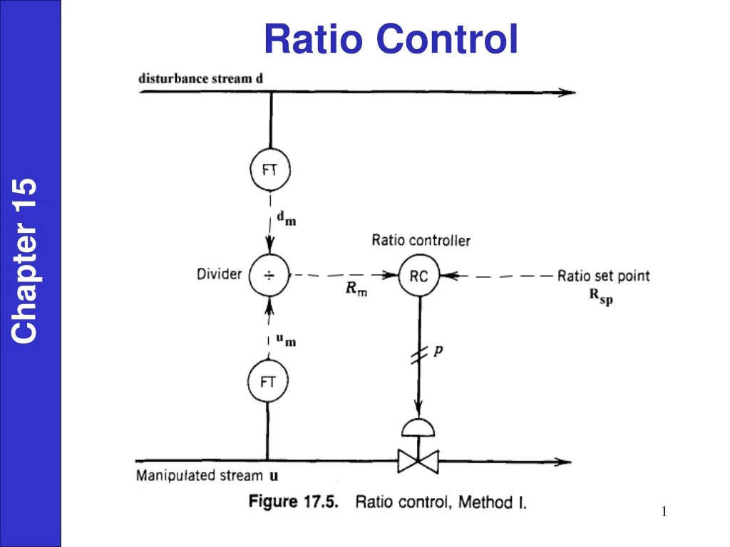
Ratio Control Chapter 15
Feedforward Control • Control Objective: Maintain Y at its set point, Ysp, despite disturbances. • Feedback Control: • Measure Y, compare it to Ysp, adjust U so as to maintain Y at Ysp. • Widely used (e.g., PID controllers) • Feedback is a fundamental concept • Feedforward Control: • Measure D, adjust U so as to maintain Y at Ysp. • Note that the controlled variable Y is not measured. Chapter 15
Feedforward vs. Feedback Control Chapter 15
Comparison of Feedback and Feedforward Control • 1) Feedback (FB) Control • Advantages: • Corrective action occurs regardless of the source and type • of disturbances. • Requires little knowledge about the process (For example, • a process model is not necessary). • Versatile and robust (Conditions change? May have to • re-tune controller). • Disadvantages: • FB control takes no corrective action until a deviation in the controlled variable occurs. • FB control is incapable of correcting a deviation from set point at the time of its detection. • Theoretically not capable of achieving “perfect control.” • For frequent and severe disturbances, process may not settle out. Chapter 15
2) Feedforward (FF) Control • Advantages: • Takes corrective action before the process is upset (cf. FB control.) • Theoretically capable of "perfect control" • Does not affect system stability • Disadvantages: • Disturbance must be measured (capital, operating costs) • Requires more knowledge of the process to be controlled (process model) • Ideal controllers that result in "perfect control”: may be physically unrealizable. Use practical controllers such as lead-lag units • 3) Feedforward Plus Feedback Control • FF Control • Attempts to eliminate the effects of measurable disturbances. • FB Control • Corrects for unmeasurable disturbances, modeling errors, etc. • (FB trim) Chapter 15
4) Historical Perspective : • 1925: 3 element boiler level control • 1960's: FF control applied to other processes EXAMPLE 3: Heat Exchanger Chapter 15
Control Objective: • Maintain T2 at the desired value (or set-point), Tsp, despite variations in the inlet flow rate, w. Do this by manipulating ws. • Feedback Control Scheme: • Measure T2, compare T2 to Tsp, adjust ws. • Feedforward Control Scheme: • Measure w, adjust ws (knowing Tsp), to control exit • temperature,T2. Chapter 15
Feedback Control Chapter 15 Feedforward Control
II. Design Procedures for Feedforward Control • Recall that FF control requires some knowledge of the process • (model). • Material and Energy Balances • Transfer Functions • Design Procedure • Here we will use material and energy balances written for SS conditions. • Example: Heat Exchanger • Steady-state energy balances Chapter 15 Heat transferred = Heat added to from steam process stream (1) Where,
Rearranging Eqn. (1) gives, (2) or (3) Chapter 15 with (4) Replace T2 by Tsp since T2 is not measured: (5)
Equation (5) can be used in the FF control calculations digital computer). • Let K be an adjustable parameter (useful for tuning). • Advantages of this Design Procedure • Simple calculations • Control system is stable and self-regulating • Shortcomings of this Design Procedure • What about unsteady state conditions, upsets etc.? • Possibility of offset at other load conditions add FB control • Dynamic Compensation • to improve control during upset conditions, add dynamic compensation to above design. • Example: Lead/lag units Chapter 15
Hardware Required for Heat Exchanger Example • 1) Feedback Control • Temp. transmitter • Steam control valve • 2) FB/FF Control • Additional Equipment • Two flow transmitters (for w and ws) • I/P or R/I transducers? • Temperature transmitter for T1 (optional) Chapter 15 Blending System Example?
EXAMPLE: Distillation Column Chapter 15 • Symbols • F, D, B are flow rates • z, y, x are mole fractions of the light component • Control objective: • Control y despite disturbances in F and z • by manipulating D. • Mole balances: F=D+B; Fz=Dy+Bx
EXAMPLE: cont. Combine to obtain Replace y and x by their set point values, ysp and xsp: Chapter 15
Analysis of Block Diagrams • Process Chapter 15 • Process with FF Control
Analysis (drop the “s” for convenience) For “perfect control” we want Y = 0 even though D 0. Then rearranging Eq. (3), with Y = 0 , gives a design equation. Chapter 15
Examples: • For simplicity, consider the design expression in the Eqn. (15-21), • then: • 1) Suppose: • Then from Equation (15-21), • 2) Let • Then from Equation (15-21) Chapter 15 (lead/lag) - implies prediction of future disturbances (15-25)
The ideal controller is physically unrealizable. • 3) Suppose , same Gd • To implement this controller, we would have to take the • second derivative of the load measurements (not possible). • Then, • This ideal controller is also unrealizable. • However, approximate FF controllers can result in • significantly improved control. • (e.g., set s=0 in unrealizable part) • See Chapter 6 for lead-lag process responses. Chapter 15 (15-27)
FF/FB Control Chapter 15
Stability Analysis • Closed-loop transfer function: Design Eqn. For GF For Y=0 and D 0 , then we require Chapter 15 previous result (15-21) • Characteristic equation The roots of the characteristic equation determine system stability. But this equation does not contain Gf. **Therefore, FF control does NOT affect stability of FB system.
Chapter 15 Figure 15.13. Comparisons of closed-loop responses: (a) feedforward controllers with and without dynamic compensation; (b) FB control and FF-FB control.
Lead-Lag (LL) Units • Commonly used to provide dynamic compensation in FF control. • Analog or digital implementation (Off the shelf components) • Transfer function: • Tune 1, 2, K If a LL unit is used as a FF controller, Chapter 15 K = 1 For a unit step change in load, Take inverse Laplace Transforms,
Step 2: Fine tune 1 and 2making small steps changes in L. • Desired response equal areas above and below set-point; small deviations Chapter 15 • According to Shinskey (1996), equal areas imply that the difference • of 1 and 2 is correct. In subsequent tuning (to reduce the size • of the areas), 1 and 2 should be adjusted to keep 1 - 2 • constant.
Step 4: Tune the FB Controller • Various FB/FF configurations can be used. • Examples Add outputs of FB and FF controllers (See previous block diagram). FB controller can be tuned using conventional techniques (ex. IMC, ITAE). Chapter 15
Chapter 15 Previous chapter Next chapter