Download
1 / 20
200 likes | 281 Views
Emmanuel Boutillon, Eric Martin LESTER, Universite de Britagne Sud Lorient, France. High-Level Design Verification using Taylor Expansion Diagrams: First Results. Maciej Ciesielski ECE Department. Univ. of Massachusetts. Priyank Kalla ECE Department University of Utah. F(x). x. ….

E N D
Emmanuel Boutillon, Eric Martin LESTER, Universite de Britagne Sud Lorient, France High-Level Design Verification using Taylor Expansion Diagrams:First Results Maciej Ciesielski ECE Department. Univ. of Massachusetts Priyank Kalla ECE Department University of Utah
F(x) x … F(0) F’(0) F’’(0)/2 Taylor Expansion Diagram (TED) • Compact, canonical representation for arithmetic functions (F: Int Int ) • Treat discrete function as continuous (polynomial) • Taylor Expansion (around x=0): F(x) = F(0) + x F’(0) + ½ x2 F’’(0) + … • Notation F(x=0) 0-child- - - - -- F’(x=0) 1-child---------- ½ F’’(x=0) 2-child====== etc. F(x) = 0-child+ x (1-child) + x2(2-child) + …
X2 = (8x3 + 4x2 + 2x1 + x0)2 (A+B)(A+2C) 64 x3 A 1 16 1 16 x2 x2 B B 8 1 4 C 4 x1 x1 2 4 1 2 1 x0 x0 1 0 1 1 1 1 0 TED – a few Examples A,B,C: arbitrary word width X decomposed in bits TED: not a BDD, not a *BMD, not a decision diagram
TED: Composition & Manipulation • Analogous to BDD and *BMD, TED: • Requires an ordering of variables • Has to be reduced • Has to be normalized • Reduced ordered normalized TED is canonical • Composition of TED: • f = g + h; APPLY(+, g, h) • f = g * h; APPLY(*, g, h) • f = g – h; APPLY(+, g, APPLY(*, -1, h))
TED: Applications and First Results • TED can represent multivariate polynomials • Possible applications • Discrete functions polynomials • RTL transformations: A*B + A*C = A*(B+C) • Algorithm specification and verifications • Experimental results
Verification Experiments:RTL Transformations A*C + B*C + A*D + B*D = (A+B)*(C+D) (arbitrary word-width)
Previous PE Computation A[ i ] B[ j ] - + Sum of Differences Array Processing FIFOs 16x16 PE Array PE 2 Previous PE Computation A[ i ] Sum 2 B[ j ] - + Sum of Differences Of squares
Array Processing PE Computation: A[ i ] – B[ j ], 8-bit vectors Effect of array size Size (# nodes) Time [s]
Verification Experiments:Array Processing 2 2 PE Computation: A[ i ] – B[ j ], 8-bit vectors Effect of array size Size ( nodes) Time [s] = out of memory
Applications to RTL Verification • Equivalence checking with TEDs • interfacing arithmetic and Boolean domains A = [an-1, …,ak,…,a0] = [Ahi,ak,Alo], B = [bn-1, …,bk,…,b0] = [Bhi,bk,Blo] B A + * F2 A F1 - 0 1 1 0 * B - * D s2 ak s1 ak D > bk bk F2 = (1-s2) (A2-B2) + s2 D s2 = ak’ bk = 1 - ak + ak bk F1 = s1(A+B)(A-B) + (1-s1)D s1 = (ak > bk) = ak (1-bk) A = 2(k+1)Ahi + 2k ak + Alo B = 2(k+1)Bhi + 2 kbk + Blo
F1 = F2 D ak ak bk bk -1 -1 Ahi 22k+2 1 Bhi 2k+2 -22k+2 Alo Alo -2k+2 Blo 2k+1 2k 2k 1 1 1 RTL Verification – cont’d. F1 = s1(A+B)(A-B) + (1-s1)D A = [Ahi, ak, Alo] B = [Bhi, bk, Blo] s1 = (ak > bk) = ak (1-bk) 0
Algebraic-Boolean InterfaceSize of TEDs vs. Boolean Logic Vary k = size of Boolean logic Time [s] Size (nodes)
A0 A1 FFT(A) A2 FAB1 IFFT0 A3 IFFT1 FAB2 InvFFT(FAB) IFFT2 FAB2 B0 IFFT3 FAB3 B1 FFT(B) B2 B3 x x x x C0 A[0:3] C1 Conv(A,B) C2 B[0:3] C3 Verification of Algorithmic Specifications
A0 A2 A1 A3 B0 • B2 B3 B1 4 0 Isomorphic TEDs: IFFT(i) Conv(i) IFFT0 = C0 = 4{ A0*B0 + A1*B3 + A2*B2 + A3*B1}
0 4 2 3 1 0 2 3 2 X X 0 4 3 = X X = Y 4 3 Y = * Y Y 2 1 4 0 3 2 1 0 1 3 1 + = 0 1 1 0 0 Applications to Galois Field Computations • Assume Galois Field GF[8], let be primitive element of GF(8) • Q[XY] = ( X + Y)( X + Y) • R[XY] = X + Y • Q[XY] = R[XY] (isomorphic TEDs)
Conclusions and Future Work • Limitations, RTL: • Increase in Boolean logic degrades performance • Internal fanouts a problem • Cannot break outputs into subfields • Applications: • RTL, behavioral, algorithmic levels • Specification and equivalence checking • Applicable to varied computational domains: integer, binary, complex, Galois Field, etc. • DSP, error correction coding, cryptography…. • Potential application: Architectural Synthesis?
Canonical Compact Linear for polynomials of arbitrary degree TED for Xk, k = const, with n bits, hask(n-1)+1 nodes *BMD is polynomial in n Can contain symbolic, word-level, and Boolean variables It is not a Decision Diagram X2 = (8x3 + 4x2 + 2x1 + x0)2 64 x3 1 16 16 x2 x2 8 1 4 4 x1 x1 4 1 2 1 x0 x0 1 1 1 1 0 Properties of TED n = 4, k = 2
Verification Experiments:Array Processing PE Computation: A[ i ] – B[ j ] A[ i ], B[ j ]:8-bit vectors
Verification Experiments:Array Processing 2 2 PE Computation: A[ i ] – B[ j ] A[ i ], B[ j ]: 8-bit vectors
Algebraic-Boolean InterfaceSize of TEDs vs. Boolean Logic Vary k = size of Boolean logic