Download
1 / 20
200 likes | 433 Views
Kerr/CFT 対応における Non- extremal 補正について. 松尾 善典. Based on YM- Tsukioka - Yoo [arXiv:0907.0303] YM- Nishioka [arXiv:1010.4549]. Kerr/CFT 対応における Non- extremal 補正について. Kerr/CFT 対応において Left mover は Extremal での エントロピーを、 Right mover は Non- extremal の補正を与える。

E N D
Kerr/CFT対応におけるNon-extremal補正について 松尾 善典 Based on YM-Tsukioka-Yoo [arXiv:0907.0303] YM-Nishioka [arXiv:1010.4549]
Kerr/CFT対応におけるNon-extremal補正について • Kerr/CFT対応においてLeft moverはExtremalでのエントロピーを、Right moverはNon-extremalの補正を与える。 • Hidden conformal symmetryの解析から、Central chargeは cL = cR = 12Jとなると予想される。 • しかし、Near horizon limitにおけるAsymptotic symmetryを用いた解析では cL = 12J,cR = 0となる。 • そこで、新しいNear horizon limitを導入する。 • この新しいNear horizon limitのもとでAsymptotic symmetryを用いてCentral chargeを計算すると cL = cR = 12Jとなる。 • このときLeft moverとRight moverそれぞれのLeading orderでのエントロピーへの寄与は、Bekenstein-Hawkingエントロピーの示唆する値と一致する。
Kerrblack hole Metric of Kerr black hole is given by ∲ ∲ ∲ ∲ ∲ ∲ ⊡ ⊢ ∽ ≲ ∲ ≍ ≲ ∫ ≡ ∻ ⊽ ∽ ≲ ∫ ≡ ≣ ≯ ≳ ⊵ ∲ ⊣ ⊤ ∲ ⊢ ≳ ≩ ≮ ⊵ ⊽ ∲ ∲ ∲ ∲ ∲ ∲ ∲ ∲ ∲ ⊡ ⊡ ⊡ ≤ ≳ ∽ ∨ ≤ ≴ ≡ ≳ ≩ ≮ ⊵ ≤ ⋁ ∩ ∫ ∨ ≲ ∫ ≡ ∩ ≤ ⋁ ≡ ≤ ≴ ∫ ≤ ≲ ∫ ⊽ ≤ ⊵ ⊡ ≲ ≲ ≍ ∲ ⊼ ≡ ≍ ≍ ≲ ∲ ∲ ⊽ ⊽ ⊢ where ⊡ ∫ ∫ ≔ ≍ ∽ ∽ ∻ ∻ ≓ ≊ ∽ ∽ ≈ ≁ ≄ ≍ ∴ ⊼ ≍ ≲ ≇ ≇ ≇ ∫ ≎ ≎ ≎ 2 parameters are related to the ADM mass and angular momentum as Temperature and entropy are given by
Near horizon limit of Kerr black hole We define near horizon coordinates as ∲ ∲ ∴ ≡ ≳ ≩ ≮ ⊵ ∲ ∲ ≦ ∨ ⊵ ∩ ∽ ≡ ∨ ∱ ∫ ≣ ≯ ≳ ⊵ ∩ ∻ ≦ ∨ ⊵ ∩ ∽ ∰ ⋁ ∲ ∲ ≤ ≲ ≞ ∱ ∫ ≣ ≯ ≳ ⊵ ⊵ ⊶ ≞ We consider near-extremal case ≞ ≞ ∲ ∲ ∲ ∲ ∲ ∲ ⊡ ⊡ ≤ ≳ ∽ ∨ ≲ ≞ ≲ ≞ ∩ ≦ ∨ ⊵ ∩ ≤ ≴ ∫ ≦ ∨ ⊵ ∩ ∨ ≤ ⋁ ∫ ≲ ≞ ≤ ≴ ∩ ∫ ≦ ∨ ⊵ ∩ ∫ ≦ ∨ ⊵ ∩ ≤ ⊵ ∰ ⋁ ∰ ∰ ≴ ≈ ∲ ∲ ≲ ≞ ∲ ⊡ ≲ ≞ ≲ ≞ ≞ ⊡ ≞ ∱ ∡ ≈ ≴ ∽ ∲ ⊲ ≡ ≴ ∻ ≲ ∽ ≡ ⊲ ∨ ∱ ∫ ∰ ⊲ ≲ ≞ ∩ ≈ ∻ ⋁ ∽ ⋁ ∫ ∲ ≍ ∽ ≡ ∱ ∫ ⊲ ∲ ≡ ∲ And take the limit of Then, the metric becomes where
Asymptotic Symmetry We first introduce a boundary condition In this case Next, we introduce perturbations of same order ⊡ ≮ ≏ ≏ ∡ ≏ ≏ ≏ ≧ ⊹ ⊱ ∫ ≧ ≧ ∨ ≨ ∽ ⋂ ⋂ ∽ ∤ ∽ ∩ ∽ ∨ ≧ ⊹ ≧ ⋂ ≲ ∨ ≧ ⊹ ∫ ⋂ ∽ ∩ ≨ ∫ ∩ ∨ ⋂ ∨ ⋂ ∩ ∩ ⊹ ⊺ ⊹ ⊺ ⊻ ⊹ ⊺ ⊹ ⊺ ⊹ ⊹ ⊺ ⊹ ⊺ ⊺ ⊻ ⊹ ⊹ ⊺ ⊹ ⊺ ⊺ ⊹ ⊹ ⊺ ⊺ ⊹ ⊺ ⊹ ⊺ ⊹ ⊺ where Then, if the metric satisfies the following condition: The geometry is asymptotically symmetric, namely,
Asymptotic symmetry for left movers For left movers, the boundary condition is given by [Guica-Hartman-Song-Strominger,’08] ≞ ≞ ≴ ≲ ≞ ⋁ ⊵ ∰ ∱ ⊳ ⊴ ⊳ ⊴ ≞ ⊡ ⊡ ∲ ∲ ∰ ∱ ≏ ≏ ≏ ≏ ≴ ∨ ≲ ≞ ∩ ∨ ≲ ≞ ∩ ∨ ≲ ≞ ∩ ∨ ≲ ≞ ∩ ≞ ≞ ⊡ ∰ ∲ ∰ ≏ ⊡ ≏ ⊻ ∽ ⊲ ∨ ⋁ ∩ ∫ ∨ ≲ ∩ ≀ ∫ ≲ ≞ ⊲ ∨ ⋁ ∩ ∫ ∨ ≲ ∩ ≀ ≂ ≃ ≞ ⊻ ≲ ≞ ≞ ⊻ ≞ ⋁ ≂ ≃ ≩ ≮ ⋁ ⊡ ⊡ ≛ ⊻ ∻ ⊻ ≝ ⊲ ∽ ∨ ⋁ ∩ ≩ ∨ ∽ ≮ ≥ ≭ ∩ ⊻ ⊡ ⊡ ⊡ ∳ ∱ ∲ ⊳ ⊴ ≏ ≏ ≏ ≲ ≞ ∨ ≲ ≞ ∩ ∨ ≲ ≞ ∩ ∨ ≲ ≞ ∩ ≂ ≃ ≮ ≭ ⊻ ≮ ∫ ≭ ≮ ≏ ∨ ⋂ ∩ ∽ ≂ ≃ ⊹ ⊺ ⊡ ⊡ ∳ ∳ ≂ ≃ ≏ ≏ ≞ ∫ ≃ ∫ ∨ ≲ ∩ ≀ ∫ ∨ ≲ ≞ ∩ ≀ ⊡ ∰ ∱ ≏ ≏ ⋁ ∨ ≲ ≞ ∩ ∨ ≲ ≞ ∩ ≞ ⊵ ≀ ≁ ≴ ⊡ ∱ ≏ ⊵ ∨ ≲ ≞ ∩ Then, the asymptotic symmetry is given by This symmetry forms the Virasoro algebra where
Asymptotic symmetry for right movers We impose the following boundary condition ≞ ≞ ≴ ≲ ≞ ⋁ ⊵ ∰ ∱ ⊳ ⊴ ⊳ ⊴ ≞ ≞ ∰ ∰ ∰ ∰ ∰ ⊲ ∨ ≴ ∩ ⊲ ∨ ≴ ∩ ≞ ⊡ ⊡ ⊡ ∰ ∳ ∲ ∳ ⊻ ⊻ ≏ ≏ ≏ ≏ ≴ ∨ ≲ ≞ ∩ ∨ ≲ ≞ ∩ ∨ ≲ ≞ ∩ ∨ ≲ ≞ ∩ ∰ ≞ ≞ ⊡ ⊻ ∽ ⊲ ∨ ≴ ∩ ∫ ≀ ∫ ≲ ≞ ⊲ ∨ ≴ ∩ ∫ ≀ ≂ ≃ ≞ ⊻ ≲ ≞ ≴ ⊻ ∲ ∲ ≲ ≞ ∲ ≲ ≞ ≂ ≃ ⊡ ⊡ ⊡ ∴ ∳ ∴ ≏ ≏ ≏ ≲ ≞ ∨ ≲ ≞ ∩ ∨ ≲ ≞ ∩ ∨ ≲ ≞ ∩ ≞ ≞ ≂ ≃ ≮ ∫ ∱ ⊡ ≛ ⊻ ∻ ⊻ ⊲ ≝ ∽ ∨ ≴ ∩ ∨ ≮ ∽ ≴ ≭ ∩ ⊻ ⊳ ⊴ ≞ ≏ ∨ ⋂ ∩ ∽ ∰ ∰ ≂ ≃ ⊲ ∨ ≴ ∩ ≮ ≭ ⊻ ≮ ∫ ≭ ⊹ ⊺ ≮ ≂ ≃ ≞ ⊻ ⊡ ⊡ ∲ ∳ ⊡ ∳ ≏ ≏ ⋁ ∨ ≲ ≞ ∩ ∨ ≲ ≞ ∩ ⊡ ≏ ∫ ≃ ≀ ∫ ∨ ≲ ≞ ∩ ≀ ≁ ≞ ⋁ ≲ ≞ ⊡ ∳ ≏ ⊵ ∨ ≲ ≞ ∩ Then, the asymptotic symmetry is given by This symmetry forms the Virasoro algebra where
Asymptotic charge Asymptotic Charge is defined as [Barnich-Brandt-Compere] ≨ ⊡ ⊢ ∱ ∱ ≾ ⊹ ⊺ ⊹ ⊺ ⊹ ⊸ ⊺ ⊹ ⊺ ⊸ ⊹ ⊺ ⊡ ≫ ≛ ≨ ∻ ≧ ⊹ ≝ ∽ ⊻ ≄ ≨ ⊻ ≄ ≨ ∫ ≄ ≨ ⊻ ∫ ≨ ≄ ⊻ ⊸ ⊸ ⊻ ∲ ∲ ≩ ⊡ ⊢ ∱ ≾ ⊹ ⊺ ⊹ ⊸ ⊺ ⊹ ⊸ ⊺ ⊺ ∲ ⊡ ⊡ ∤ ≨ ≄ ⊻ ∫ ≨ ∨ ≄ ⊻ ∫ ≄ ⊻ ∩ ∨ ⊹ ⊺ ∩ ≫ ≛ ≨ ∻ ≧ ⊹ ≝ ∽ ≫ ≛ ≨ ∻ ≧ ⊹ ≝ ≤ ≸ ≚ ≚ ≚ ≚ ⊸ ⊸ ⊸ ⊻ ∲ ⊻ ⊹ ⊺ ∱ ∱ ∱ ∱ ≣ where ∳ ⊡ ≏ ⊱ ≑ ∽ ≫ ≑ ≛ ≛ ∤ ≨ ≝ ≫ ∽ ≧ ⊹ ≛ ∻ ∤ ≧ ⊹ ≝ ≧ ⊹ ∽ ∻ ≧ ⊹ ≝ ∫ ≩ ⊱ ≫ ≛ ≨ ∻ ≮ ≧ ⊹ ≝ ≫ ≛ ∫ ∤ ≨ ∻ ∨ ≮ ≧ ⊹ ≝ ∩ ⊳ ⊻ ⊻ ⊻ ⊻ ⊻ ⊳ ≮ ∫ ⊻ ≭ ∻ ∰ ⊻ ⊳ ≮ ≭ ∸ ⊼ ≇ ∸ ⊼ ≇ ∸ ⊼ ≇ ∸ ⊼ ≇ ∱ ∲ ≎ ≎ ≎ ≎ ≀ ⊧ ≀ ⊧ ≀ ⊧ ≀ ⊧ We consider transform of the charge itself The central charge can be read off from the first term
Central charges For left movers, we obtain ≚ ≚ ∱ ∲ ∲ ∱ ∱ ∲ ≡ ≡ And for right movers, ≫ ≛ ∤ ≧ ⊹ ∻ ≧ ⊹ ≝ ∽ ∰ ∳ ⊻ ⊡ ≣ ∽ ≫ ≛ ∤ ≧ ⊹ ∻ ∱ ≧ ⊹ ∲ ≝ ≊ ∽ ∻ ≩ ⊱ ∨ ≣ ≮ ∽ ∫ ∰ ∲ ≮ ∩ ⊻ ⊻ ≌ ⊻ ⊻ ≮ ∫ ≭ ∻ ∰ ≒ ≮ ≭ ∸ ⊼ ≇ ≮ ≭ ∸ ⊼ ≇ ≇ ≇ ≎ ≀ ⊧ ≎ ≎ ≎ ≀ ⊧ Then, the central charges become
Cardy formula and entropy Frolov-Thorne temperature is defined as • For left mover, the Cardy formula reproduce the entropy of the extremal Kerr black hole. • For right mover, we obtain cR = 0, and does not contribute to the entropy. ⊷ ⊸ ⊷ ⊸ ∱ ≲ ≞ ∲ ∲ ∲ ∡ ⊭ ≮ ≮ ⊼ ⊼ ∲ ⊼ ≡ ≈ ≈ ≌ ≒ In this case, we obtain ≔ ∽ ∻ ≔ ∽ ⊡ ⊡ ⊡ ≥ ≸ ≰ ∫ ≭ ∽ ≥ ≸ ≰ ≓ ∽ ≣ ≔ ∫ ≣ ≔ ∽ ≌ ≒ ≌ ≌ ≒ ≒ ∲ ⊼ ∲ ⊼ ≔ ≔ ≔ ≔ ∳ ∳ ≇ ≈ ≈ ≌ ≒ ≎ By using the Cardy formula,
Quasi-local charge Quasi-local charge is defined in a similar fashion to the GKPW We first define the surface energy-momentum tensor ≚ ≰ ∱ ∲ ⊱ ≓ ≧ ≲ ≡ ≶ ∲ ⊹ ⊹ ≣ ⊹ ≴ ⊺ ≰ ⊡ ⊡ ⊡ : Induced metric ≔ ≑ ∽ ∽ ≔ ⊿ ∽ ∽ ≤ ≋ ≸ ≔ ⊾ ⊰ ≵ ⊻ ∨ ≋ ⊾ ≔ ≵ ⊰ ⊿ ⊻ ≋ ∩ ⊹ ⊺ ⊻ ⊹ ⊹ ⊺ ⊺ ⊹ ⊹ ⊹ ⊹ ⊺ ⊺ ⊺ ⊺ ⊹ ⊺ ⊹ ⊹ ⊺ ⊺ ⊹ ⊺ ⊡ ∸ ⊼ ≇ ⊰ ⊱ ⊰ ≎ ⊹ ⊺ For Einstein gravity, it can be written as : extrinsic curvature We regularize the surface energy-momentum tensor as The quasi-local charge is defined by : timelike unit normal : Killing vector : Induced metric on timeslice at boundary
Cardy formula for right mover The central charge can be read off from the anomaly ≲ where we put the boundary at ≲∽⊤. ∲ ∲ ∲ ≡ ∱ ≡ ∲ ≡ ⊹ ∲ ∲ ≣ ≌ ∨ ∲ ⊼ ∩ ≡ ≔ ⊹ ∰ ∰ ∰ ∲ ≒ ∰ ≌ ∽ ⊱ ≑ ≍ ≣ ∽ ∽ ∽ ⊲ ∨ ∨ ∲ ≴ ⊼ ∩ ≔ ∩ ≓ ∽ ∲ ⊼ ∽ ∰ ⊻ ≒ ⊻ ≇ ∲ ≇ ≇ ⊤ ⊤ ⊤ ∶ ≇ ⊤ ≎ ≎ ≎ ≎ Then, the central charge is For finite temperature, we obtain Then, the Cardy formula gives
Non-extremal correction By using the Frolov-Thorne temperature, • The Cardy formula gives the non-extremal correction of the entropy, if we identify . • If is kept finite, the geometry is approximated by near horizon geometry in near horizon region . • The boundary of the near horizon geometry should be taken around . Therefore, we identify . ∲ ∲ ∲ ⊼ ≡ ∲ ⊼ ≡ ≲ ≞ ∮ ⊡ ∱ ≈ ⊡ ⊿ ≲ ⊤ ⊤ ≲ ≞ ∽ ∽ ≲ ⊲ ∱ ∱ ∽ ∽ ⊲ ⊲ ≡ ⊢ ⊢ ⊢ ≓ ∽ ≓ ∽ ∨ ∱ ∫ ⊲ ≲ ≞ ∫ ∩ ∫ ≈ ≇ ≇ ⊤ For near-extremal case, the entropy is ≎ ≎ ⊲
Hidden Conformal Symmetry [Castro-Maloney-Strominger’10] We consider the scalar field in Kerr background. ⊷ ⊸ ∲ ∲ ⊡ ⊡ ∨ ∲ ≍ ≲ ∡ ≡ ≭ ∩ ∨ ∲ ≍ ≲ ∡ ≡ ≭ ∩ ⊡ ∫ ∲ ∲ ∲ ⊡ ≀ ⊢ ≀ ∫ ∫ ∨ ≲ ∫ ∲ ≍ ≲ ∫ ∴ ≍ ∩ ∡ ≒ ∨ ≲ ∩ ∽ ≋ ≒ ∨ ≲ ∩ ≲ ≲ ⊡ ⊡ ⊡ ⊡ ∨ ≲ ≲ ∩ ∨ ≲ ≲ ∩ ∨ ≲ ≲ ∩ ∨ ≲ ≲ ∩ ⊡ ⊡ ⊡ ∫ ∫ ∫ ⊷ ⊸ ∲ ∲ ⊡ ⊢ ⊡ ⊡ ≰ ∨ ∲ ≍ ≲ ∡ ≡ ≭ ∩ ∨ ∲ ≍ ≲ ∡ ≡ ≭ ∩ Then, the scalar field can be factorized as ⊡ ∫ ⊡ ⊡ ≀ ⊢ ≀ ∫ ≒ ∨ ≲ ∩ ∽ ≋ ≒ ∨ ≲ ∩ ⊹ ⊺ ≩ ∡ ≴ ∫ ≩ ≭ ⋁ ⊡ ⊩ ≀ ∨ ≴ ∻ ≲ ∻ ⋁ ∻ ≧ ⊵ ≧ ∩ ∽ ≀ ≥ ⊩ ∨ ≴ ∻ ≲ ∻ ⋁ ∻ ≒ ⊵ ∩ ∨ ≲ ∩ ∽ ≓ ∨ ∰ ⊵ ∺ ∩ ≲ ≲ ⊹ ⊺ ⊡ ⊡ ⊡ ⊡ ∨ ≲ ≲ ∩ ∨ ≲ ≲ ∩ ∨ ≲ ≲ ∩ ∨ ≲ ≲ ∩ ⊡ ⊡ ⊡ ∫ ∫ ∫ EOM for radial part of Scalar in Kerr background For small ∡, this equation can be approximated as
We define conformal coordinates as ≲ ≲ ⊡ ⊡ ≲ ≲ ≲ ≲ ≴ ∫ ∫ ⊡ ⊡ ∫ ∲ ⊼ ≔ ⋁ ∲ ⊼ ≔ ⋁ ≷ ∽ ≥ ∻ ≷ ∽ ≥ ∻ ≒ ≌ ∲ ≍ ⊡ ⊡ ≲ ≲ ≲ ≲ ⊡ ≲ ∫ ≲ ≲ ≲ ∲ ∲ ∨ ∲ ≍ ≲ ≀ ∫ ≡ ≀ ∩ ∨ ∲ ≍ ≲ ≀ ∫ ≡ ≀ ∩ ⊡ ⊡ ⊡ ⊡ ∫ ∫ ≲ ⊡ ∫ ≴ ⋁ ≴ ⋁ ≔ ∽ ∻ ≔ ∽ where ⊡ ≀ ⊢ ≀ ∫ ≩ ≩ ⊡ ≲ ≲ ≌ ≒ ≲ ≲ ≴ ⊡ ∫ ∴ ⊼ ≡ ∴ ⊼ ≡ ⊡ ⊼ ∨ ≔ ∫ ≔ ∩ ⋁ ⊡ ⊡ ⊡ ⊡ ∨ ≲ ≲ ∩ ∨ ≲ ≲ ∩ ∨ ≲ ≲ ∩ ∨ ≲ ≲ ∩ ≹ ∽ ≥ ∻ ≒ ≌ ∴ ≍ ⊡ ⊡ ⊡ ∫ ∫ ∫ ⊡ ≲ ≲ ⊡ ∱ ∱ ∳ ∲ ∽ ≹ ≀ ≀ ∫ ≹ ≀ ≀ ⊡ ≹ ≹ ∫ ∴ ≹ Then, the laplacian becomes that on AdS3 .
HCS and BTZ black hole In the Kerr background, ⋁ has a periodicity ⊷ ⊵ ⊶ ⊸ ∲ ∲ ⊡ ∱ ∴ ≡ ≲ ∫ ≲ ∨ ≲ ≲ ∩ ⊡ ⊡ ∫ ∫ ∲ ∲ ∲ ∲ ⊡ ⊡ ⊡ ≀ ⊢ ≀ ∫ ≲ ≀ ≀ ≡ ≀ ≡ ≀ The approximated background is not equivalent to the AdS3, but its quotient. ≡ ⊡ ≲ ≲ ∫ ⊡ ∫ ∲ ⊢ ≲ ∫ ≲ ∲ ∨ ≲ ∫ ≲ ∩ ⊡ ∫ ⊡ ≸ ∽ ⋁ ∻ ≸ ∽ ⋁ ≴ ⊡ ⊡ ∫ ∫ ∲ ⊻ ⋁ ⋁ ∫ ∲ ⊼ ∲ ≍ BTZ black hole We define the “light-cone” coordinates as Then, the “laplacian” for radial part becomes
The metric of the BTZ black hole can be written as ⊷ ⊵ ⊶ ⊸ The Frolov-Thorne temperatures are given by ⊵ ⊶ ∲ ⊡ ∴ ∱ ∴ ≲ ∫ ≲ ∨ ≲ ≲ ∩ ∲ ∲ ∲ ∲ ∲ ∲ ∲ ∲ ⊡ ⊡ ∫ ∫ ⊡ ⊡ ∨ ⊽ ≲ ∩ ∨ ⊽ ≲ ∩ ≬ ⊽ ≤ ⊽ ≲ ≲ ∲ ∲ ⊡ ⊡ ⊡ ≀ ⊢ ≀ ∫ ≲ ≀ ≀ ≀ ≀ ⊡ ∫ ⊡ ∫ ⊡ ∲ ∲ ∲ ≲ ∫ ≲ ≲ ≲ ⊡ ≲ ≲ ∫ ⊡ ⊡ ≤ ≳ ∽ ≤ ⊿ ∫ ∫ ⊽ ≤ ∧ ≤ ⊿ ⊡ ∫ ∲ ∲ ⊡ ⊡ ∫ ∫ ≬ ⊢ ≲ ∫ ≲ ∲ ∨ ≲ ∫ ≲ ∩ ⊧ ∲ ⊧ ⊡ ≸ ≔ ∽ ∧ ∽ ⊿ ∻ ∻ ⊽ ∽ ∨ ≲ ≔ ∫ ∽ ≲ ∩ ≲ ≲ ≲ ∲ ∲ ∲ ∲ ∲ ∲ ⊡ ⊡ ⊡ ⊡ ∫ ∫ ⊽ ∨ ⊽ ≲ ∩ ∨ ⊽ ≲ ∩ ⊽ ⊡ ⊡ ≌ ∫ ≒ ∫ ⊡ ∫ ∲ ⊼ ≬ ∲ ⊼ ≬ ≬ ∽ ∲ ≡ By introducing the following coordinates The laplacian in the BTZ background is expressed as Therefore, the approximated laplacian on Kerr geometry equals to that in BTZ if we identify
New near horizon limit We define new near horizon coordinates as ⊳ ⊴ ⊳ ⊴ ⊳ ⊴ ∰ ∰ ∰ ∰ ∰ ∰ ∰ ∫ ∫ ∫ ⊲ ∨ ≸ ∩ ⊲ ∨ ≸ ∩ ⊲ ∨ ≸ ∩ ⊻ ⊻ ⊻ ∰ ⊡ ∫ ∫ ∳ ⊡ ⊡ ≏ ⊻ ∽ ⊲ ∨ ≸ ∩ ∫ ≀ ∫ ≲ ≞ ⊲ ∨ ≸ ∩ ∫ ≀ ∫ ≃ ≀ ∫ ∨ ≲ ≞ ∩ ∲ ≤ ≲ ≞ ⊡ ⊻ ∫ ≲ ≞ ⊻ ∲ ∲ ≲ ≞ ∲ ≲ ≞ ≲ ≞ ⊡ ∲ ∲ ∲ ∫ ∲ ∫ ∲ ∲ ⊡ ⊡ ≤ ≳ ∽ ∨ ≲ ≞ ≲ ≞ ∩ ≦ ∨ ⊵ ∩ ∨ ≤ ≸ ∩ ∫ ≦ ∨ ⊵ ∩ ∨ ≤ ≸ ∫ ≲ ≞ ≤ ≸ ∩ ∫ ≦ ∨ ⊵ ∩ ∫ ≦ ∨ ⊵ ∩ ≤ ⊵ ≡ ≴ ∰ ⋁ ∰ ∰ ≈ ∲ ∲ In the near horizon limit, the metric becomes ⊡ ≲ ≞ ≲ ≞ ⊡ ∫ ⊡ ≸ ∽ ⊲ ⋁ ∻ ≸ ∽ ⋁ ∻ ≲ ∽ ≡ ∨ ∱ ∫ ⊲ ≲ ≞ ∩ ≈ ∫ ⊡ ⊡ ∫ ∫ ∫ ≩ ≮ ≸ ∽ ⊲ ⊻ ⊻ ∲ ≸ ≸ ∫ ∲ ⊲ ⊼ ≮ ∨ ⊲ ≸ ∻ ∩ ∽ ⊲ ≥ ≸ ≸ ∫ ∲ ⊼ ≮ ∲ ≍ ⊻ ≮ This geometry has the following periodicity The asymptotic symmetry for right mover is which should be expanded as
Entropy Integrating on a time-slice, the following component contributes to the central charge: ⊡ ≲ ≲ ≲ ≞ ≲ ∫ ≲ ∱ ≚ ⊡ ⊡ ∫ ≈ ∫ ∡ ∡ ≔ ∽ ⊲ ∻ ≔ ∽ ∲ ∲ ∲ ∲ ∲ ⊼ ∱ ⊼ ∱ ∲ ≡ ∲ ⊼ ≡ ∲ ≡ ⊼ ≍ ≲ ⊡ ∫ ∴ ⊼ ≡ ∲ ⊼ ∴ ⊼ ≡ ∲ ⊼ ∫ ≾ ⊡ ≲ ∫ ∳ ⊻ ≓ ∽ ≣ ≔ ∫ ≫ ≣ ≛ ≣ ∤ ≔ ∽ ≧ ⊹ ∻ ∽ ≧ ⊹ ≝ ≤ ≸ ∽ ≤ ⊵ ∨ ≣ ∱ ∽ ∫ ⊱ ⊲ ≲ ≞ ∩ ≮ Then, the central charge becomes ≌ ≌ ≒ ≒ ⊻ ≒ ≌ ≮ ∫ ≈ ≭ ∻ ∰ ⊻ ≮ ∸ ⊼ ∳ ≇ ∳ ≇ ≇ ≇ ≇ ≭ ≎ ≎ ≎ ≎ ≎ ≀ ⊧ The Frolov-Thorne temperatures are given by The entropy can be reproduced by Cardy formula
Conclusion and outlook • We define a new near horizon limit. By using this limit, we obtain the central charge cL = cR = 12J. • This new definition corresponds to a modification of the asymptotic symmetry. • There are higher order corrections from metric and Killing vectors of the asymptotic symmetry. • Left movers gives O(ε0)contributions but right movers gives O(ε). • To be exact, we have calculated only the leading term for left and right movers, respectively. • They agree with the expected result. • However, the next-to-leading term from the left movers is at the same order to the leading term from right movers. • It is left to be checked that this term vanishes.