Download
1 / 22
230 likes | 400 Views
Compartments for Beginners: Wellbore Formation Testing in the Real World. SPWLA WFT SIG Houston , Texas September 27, 2011. Why are we talking about this?. What has been the outcome of the last few years of data collection?

E N D
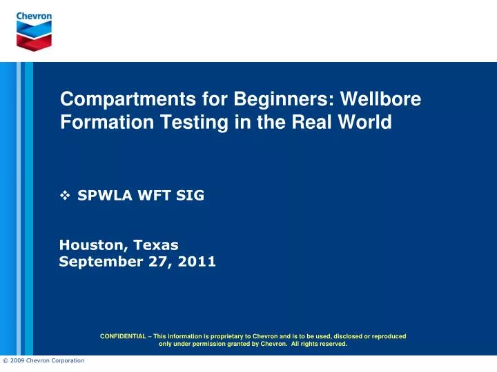
Compartments for Beginners: Wellbore Formation Testing in the Real World SPWLA WFT SIG Houston, Texas September 27, 2011
Why are we talking about this? • What has been the outcome of the last few years of data collection? • Compartments, Compartments and … more Compartments • How do we define the Value Proposition? • Importance of Sample Quality and Volume • Value of Information vs cost and risk • How do we plan and run the job? • Practical tips for adding value with new technology
The deepwater Appraisal problem:Reduce Subsurface Uncertainty in a cost-effective manner • Industry moving towards: • Ultra deepwater, deeper objectives • Non-amplitude and subsalt prospects • Less forgiving smaller targets • Appraisal problem is getting more difficult • Increased subsurface uncertainty • High appraisal costs makes reducing uncertainty expensive • $10MM to $30MM/well in deeper waters (data collection only). • Need to reduce subsurface uncertainty in a cost-effective way • Combining reservoir engineering and geochemistry in a valuable way to decide what data to collect for what cost and what is the acceptable risk to get this data
2009 DEEPSTAR 9702 Appraisal Lookback: 28 DWGOM Fields Two fields significantly outperformed expectations Six fields significantly underperformed expectations Of the remaining 22 fields 75% marginally underperformed and 25% marginally outperformed In general, fields showed more complexity than anticipated BAD RESERVES OUTCOME GOOD UGLY BAD PRODUCTION OUTCOME
Looking for Value • Why are we talking about this? • Optimize Cost and Maximize Value • Apply Appropriate FEL • For a new field discovery • Uncertainty Management Plan • Assess the impact of fluids properties on project execution • Impact of compartments on Appraisal program Compartments Fluids Impact • IMPACT • Exploration: • What is the likely value of this discovery? (oil quality and continuity) • How high a priority should this prospect get in the Appraisal Queue? • Development: • What are the “game changers”? • Effect on project architecture and selection of development options?
Compartments, Compartments and More Compartments • Compartment Risk will be determined based on how well: • Pressure trends for major and minor sands correlate over the field, • Pressure trends correlate vertically within each zone in each well, • How measured and theoretical fluid gradients compare, • How fluid properties correlate over the field (both PVT and bulk properties), and • A review of geochemical marker results. • Oil Fingerprinting • Mud gas Isotope Analysis • Solution Gas Isotope Analysis • Sulfur Isotope Analysis Real-time techniques that are useful in the timeframe needed to make decisions to complete or sidetrack are limited.
Exploration and Appraisal ActivitiesData Collection and Integration Toolkit Courtesy Arild Fossa, PowerWell Services 1 cm 1 m 1 km GEOLOGY SEISMIC Static CORES LOGS NEW PARADIGM: THE DISTRIBUTION OF PRESSURE AND FLUIDS IN THE RESEVOIR REPRESENTS A TYPE OF DYNAMIC DATA! Distance of investigation WFT PRESSURES FLUID PROPERTIES & GEOCHEMISTRY Dynamic WELLTEST TRACERS 10-2 m 10-1 m 1 m 10 m 102 m 103 m 104 m
In the Appraisal and Development PhaseHow much sample do we need and why? • We need multiple fluid samples from different wells because spatial variations in fluid composition can reflect: • Faulting, compartmentalization and reservoir architecture • Filling history as an indication of geologic complexity • Proximity to fluid contacts and gravitational grading • Biodegradation, tar mats, loss of light ends and mixing events • and allow production allocation or mechanical troubleshooting with fingerprints Water Samples: (500 to 1,000 cc per zone) • Hydrate formation, Scale, Souring and Corrosion potential, Salinity Tahiti Field: Four conventional cores, over 500 pressure points, 33 fluid samples, M-21 Well Test OWC 3 miles Geochemical allocation of fluids during the Tahiti Well Test by Russ Kaufman and Stan Teerman Relationship of optical density during Tahiti sample pumpouts with column height by Soraya Betancourt (SLB)
In the Exploration and Appraisal Phase How much sample do we need and why? • We need multiple sample bottles at each sample point because: • 300 cc sample => minimum evaluation • Samples compromised during transfer or leakage during storage • Custody transfer and inventory mistakes • Multiple measurements required for confidence • Studies that usually require substantial volumes of oil (gallons, barrels): • Restored state core floods for SCAL • Completion/stimulation fluid compatibility • Flow loop testing • Emulsions key for oils <20 deg API • Larger volumes needed (1 Bbl) From SPE 49067: “Identifying and Meeting the Key Needs for Reservoir Fluid Properties A Multi-Disciplinary Approach” B.J. Moffatt and J.M. Williams Deepwater Project Learning: Major Capital Projects relying on Wellbore Formation Tester sample volumes are typically short of STO and live fluid prior to completion of all desired experiments.
In the Exploration and Appraisal PhaseHow much sample do we need and why? Optimum Samples Volume needed for:Target: • PVT for reservoir and fluid flow simulation: GOR, Bo, density, viscosity • Volume: 1,000 cc Res Fluid / zone affect OOIP, rate and recovery • Geochemistry fingerprinting: Reservoir continuity and variability • Volume: 50 cc STO / zone Source rock typing, analogs • Hydrates, wax & asphaltene potential: Operability, cost, • Volume: 100 to 200 cc Res Fluid / zone development options • Crude Value: Market Value, STO properties • Volume: 10 gallons STO / zone and character, refinery options • Emulsion / Foaming: Viscosity variation with water cut; • Volume: 10 gallons STO / zone separation time; foam stability • Chemical Screening: Effectiveness of • Volume: 10 gallons STO select chemicals
Pour point decreases for some oils Wax appearance point decreases slightly (may be within meas. uncertainty) Saturates increase (n-Paraffins) Asphaltenes become more stable How clean does it need to be?Oil Based Mud Contamination Oil-based mud and hydrocarbon additives to water based muds can contaminate fluid samples, affecting the results of PVT and STO testing. • Plan sampling program to minimize contaminants. • Quantify the OBM components and correct for their effect. • Make sure you capture relevant OBM samples. Consider contamination of your sample from other zones (or other wells). • Until recently most OBM were 2-3 component mixtures. NovaPlus, Petrofree, Petrofree LE were C14,C16,C18, C20 mixes. Current use of ‘fillers’ makes filtrates more ‘complicated’. These are now multi-component fluids in the C7-C30 range and this makes corrections more difficult. Tahiti Field: OBM contamination corrections OBM Contamination effects: • Dew point and bubble point decrease • GOR decreases • Liquid density generally decreases • Viscosity increases
How clean does it need to be?For Black Oils: Tahiti Field: Fluid modeling of OBM contamination effects by Kathy Greenhill and Jeff Creek • PVT relationships, Density, GOR • No analogs: Target 5% OBM • Analogs available: Target 10% OBM, preferably <5% OBM. These properties can be modeled with some confidence up to 20% OBM. However, note that many labs have difficulty quantifying OBM contamination amounts above 15% OBM. • Volumetric Properties readily corrected (Rs, Bo, Do) • Saturation Pressure correction difficult (Pob, Pod) • Viscosity • Correction for OBM complicated • Experimental error with perfect sample is +/-15%. • Consider making several determinations with different OBM amounts • Flow Assurance • Wax appearance typically invariant up to 25% OBM • Asphaltene Onset Pressure variation can be significant above 10% OBM.
How clean does it need to be?For Black Oils: • Bulk fluid properties (viscosity, emulsions, assays) • Volumetric property correction for contamination is generally straightforward. • Affect on emulsions and rheology are less predictable and typically require physical testing. • Geochemistry • OBMs alter Vitrinite reflectance, TOC, density, isotopes, SARA and biomarkers. • For Black Oils, high definition studies work best when less than 10% OBM. Recent results indicate much improved results below 5% OBM. • Useful information can be obtained up to 30% OBM contamination. For Light Oils and Gas Condensates: • OBM contamination may interfere with critical light components making the acquisition of cleaner samples necessary. For difficult sampling operations, a well test may be required.
What's the best way to get the sample we need? (highest Possibility of Success, Lowest Cost) • Determine what is the likely pump-out duration • What is the overbalance? • What is the mud system (invasion profile)? • What is the expected formation / fluid mobility? • What is the anticipated fluid type (viscosity and GOR)? • Determine sampling strategy • Plan pump-out until we get to below 5% OBM contamination? Would 10% OBM be acceptable? • Consider setting maximum pump-out time (5 to 8 hours?) • Consider contingency plan • How long to pump at one station before moving? • How many attempts will be made?
What's the best way to get the sample we need? (highest Possibility of Success, Lowest Cost) • Define Risk: • Determine probability of getting tool differentially stuck • How long has the hole been open? • What is the well angle to the angle of formation bedding dip? • What is the mud system? • What is the overbalance pressure? • Indicators • Did the drill pipe take any drag on the trip out? • What does the caliper show? Does the hole have ledges or breakouts? Hole geometry is your biggest concern! • Determine the probability of getting line stuck (key seated) • What is the dog leg severity of the hole above the sampling interval? • How much formation is open above the sampling interval? • What is the overbalance in these shallower zones?
What's the best way to get the sample we need? (highest Possibility of Success, Lowest Cost) • VOI Example: Knotty Head Exploration Sampling • Exploration prospect, some well sampled zones, some under sampled zones. Developed sample acquisition hierarchy, sampling fluids in sidetrack. • Strategy – pump-out until <5% OBM contamination • Conditions… ** $3.1 Million Successful fish Yes Fish or no Fish * Loss of wellbore for further Data acquisition Yes No * Tool Stuck $4.3 Million Sampling Strategy Yes ** Would you do a VSP or RSWC ops in the same hole you just fished? No * $1.7 Million MDT tool selection <5%OBM No $0.5 Million MRPQ Off wall after 6hrs $0.35 Million Decision Uncertainty Norm probe
Chevron/Schlumberger Compartmentalization Study using Downhole Fluid Analysis at Tahiti Chevron provided both live and dead M21 Sand oil samples and the conceptual geologic framework models for each sand. Schlumberger conducted Lab VIS-NIR (using the world’s best mass spectrometer at Florida State University) and fluorescence spectroscopy (with Wood’s Hole Oceanographic Institute) on live and dead oil samples, then compared the results with field Downhole Fluid Analysis optical data. The Team successfully defined the asphaltene gradient in the oil column and tested for compartmentalization. We found small variations in GOR but large variations in Color that correlate very well with SARA Asphaltene content. Also, we found that the two-fold variation in color is a reflection of an asphaltene gradient in the oil column. The M21A and B Sands had different trends, but no clear indication of lateral compartmentalization was found.
Stratigraphy and Structure Pressures Fluid Properties Oil Geochem Solution Gas Geochem S N Mud Gas Isotopes Tahiti Field: Compartmentalization Analysis • All these methods all seem to agree that for the main Tahiti reservoir, compartments either do not exist or are limited to “baffles” • After the field came on production in April, 2009 interference was seen between all six wells within about 12 days
Tahiti Asphaltene Concentration Model Schlumberger: Nicolas Ebele, Sandra Quental, Francois Dubost, Soraya Betancourt PS003 PS03 Asphaltene Content %w/w PS002 - 640#2 ST1 BP1 640#2 ST0 BP2 Dz=1870’ a=45o + M21A Existing Wells 640#2 ST1 BP1 640#2 ST0 BP2 M21B New Wells PS002 PS003 Calibrated model with existing wells Predict DFA Optical Densities and Asphaltene Concentration in new wells drilled updip N
Sampling Best Practices • 1) Early Involvement in sample planning!!! • Try to influence mud selection and encourage minimum overbalance. Overbalance influences pump selection and pump stroke volume (which can lead to significantly longer pumpout times to displace the same volume). • Set casing over any low pressure sands, if practical. If not practical, consider conducting contingent wireline runs prior to reaching TD. • Quartz pressure gauges are very accurate. Depth control isn’t. Plan accordingly. • 2) Consider likely mobility and possible pump out times. • In general, OBM contamination is directly proportional to pumpout volume. Real-time optical analyzers are necessary to develop a feeling for sample quality and determine that pumpouts are proceeding as planned. Don’t waste rig time. • Make sure you capture a set of relevant OBM samples. • 3) Construct sampling strategy and consider the probability of tool sticking. • Consider tool selection and string weight. Build a flexible plan. Monitor drilling and consider how changing hole conditions may change risk leading up to job. • Define back-off points as clearly as possible before the job and have a clear chain of command relationship defined with Drilling. 4) Immediately after the job, QA/QC the data and properly archive the run.
Notable References for further reading: • Brown, Alton “Improved Interpretation of Wireline Pressure Data” AAPG Bulletin, v. 87 No 2 (February 2003), pages 295-311. • Brooks, A., Wilson, H., Jamieson, A., McRobbie D.,Holehouse, S.G., “Quantification of Depth Accuracy”, Paper SPE 95611 presented at the 2005 SPE Annual Technical Conference and Exhibition, Dallas, TX, U.S.A., 9-12 October. • Hashem, M., Elshahawi, H., Ugueto, G., “A Decade Of Formation Testing – Do’s and Don’ts and Tricks of the Trade”, SPWLA Paper 2004L, presented at the SPWLA 45th Annual Logging Symposium Noordwijk, The Netherlands, 6-9 June, 2004. • Kabir, C.S., Pop, J.J., “How Reliable is Fluid Gradient in Gas/Condensate Reservoirs?”, Paper SPE 99386, presented at the SPE Gas Technology Symposium held in Calgary, Alberta, Canada, May 14-17, 2006. • Lee, J., Michaels, J., Shammai, M., Wendt, W., “Precision Pressure Gradient Through Disciplined Pressure Survey”, SPWLA Paper 2003EE, presented at the SPWLA 44th Annual Logging Symposium, Galveston, Texas, U.S.A., 6-9 June, 2003. • Mullins, Oliver C., Betancourt, Soraya S., Cribbs, Myrt E., Creek, Jefferson L., Dubost, Francois X. Dubost, Andrews, A. Ballard and Venkataramanan, Lalitha, “Asphaltene Gravitational Gradient in a Deepwater Reservoir as Determined by Downhole Fluid Analysis” SPE 102571 presented at the SPE International Symposium on Oilfield Chemistry held in Houston, Texas, U.S.A., 28 February–2 March 2007. • Charles Collins, Mark Proett, Bruce Storm and Gustavo Ugueto, “An Integrated Approach to Reservoir Connectivity and Fluid Contact Estimates by Applying Statistical Analysis Methods to Pressure Gradients”, paper presented at the SPWLA 48th Annual Logging Symposium held in Austin, Texas, USA, 3-6 June, 2007. • Elshahawi, M. Hashem, D. McKinney and M. Flannery, Shell, L. Venkataramanan and O. C. Mullins, Schlumberger, “Combining Continuous Fluid Typing, Wireline Formation Tester and Geochemical Measurements for an Improved Understanding of Reservoir Architecture”, SPE 100740, paper presented at the 2006 SPE Annual Technical Conference and Exhibition, San Antonio, Texas, U.S.A., 24-27 September. • Elshahawi, H., Samir, M., Fathy, K.,, “Correcting for Wettability and Capillary Effects on Formation Tester Measurements”, SPWLA Paper 2000R, presented at the SPWLA 41st Annual Logging Symposium, June 4-7. • Asphaltenes, Heavy Oils, and Petroleomics, Oliver Mullins, et al. (eds.), Springer, 2007