Download
1 / 82
820 likes | 977 Views
Guessing Attacks in the pi-calculus. (Work in progress). Tom Chothia École Polytechnique. Outline of Talk. Background: Formal security in the pi-calculus. Computational arguments. Bridging the gap. The pi-calculus with guessing. Calculating the cost of a guessing attack.

E N D
Guessing Attacks in the pi-calculus (Work in progress) Tom Chothia École Polytechnique
Outline of Talk • Background: • Formal security in the pi-calculus. • Computational arguments. • Bridging the gap. • The pi-calculus with guessing. • Calculating the cost of a guessing attack. • The computational correctness of the calculus
pi-g Summary : • A pi-calculus extended with primitives for guessing and tracking the effects of the guess. • A method of scoring traces in the calculus to show how hard that “attack” would be using guesses and multiple tries. • With most of the simplicity of formal methods and some of the power of computational methods.
Pi-calculus Process P,Q,A ::= 0 | send a b | rec a b;P | ! P | new a;P | ( P | Q ) | [a=b]; P
Pi-calculus Key reduction rules: ( send a b | rec a x;P ) -> P [ b/x ] new a;( P ) | Q = new a;( P | Q ) if “a” not free in Q N.B. “send a b | ( new a; rec a x; P)” cannot communicate.
Pi-calculus • Analyse a process P with message M. • An attacker is any context: C[P(M)] • If for all M’ we have P(M) is weakly bi-similar P(M’) then M is secure in P. • N.B. weak bi-simulation is a congruence for the spi-calculus • So above condition implies that for all hostile attackers A, A[P(M)] is weakly bi-similar to A[P(M’)].
Pi-calculus example A(M) = new cAB send cAS cAB; send cAB M S = rec cAS x; send cBS x B = rec cSB x ; rec x y;F(y) A S B
Pi-calculus example A(M) = new cAB send cAS cAB; send cAB M S = rec cAS x; send cBS x B = rec cSB x ; rec x y;F(y) Inst(M) = new cAS; new cBS;( A(M) | S | B) Secrecy: M and M’ Inst(M) ~ Inst(M’) iff F(M) ~ F(M’)
Pi-calculus example A(M) = new cAB send cAS cAB; send cAB M S = rec cAS x; send cBS x Bspec = rec cSB x ; rec x y;F(M) Instspec(M) = new cAS; new cBS;( A(M) | S | Bspec) Secrecy: M and M’ Inst(M) ~ Inst(M’) iff F(M) ~ F(M’) Authenticity: M : Inst(M) ~ Instspec(M)
Spi-calculus • The spi-calculus adds encryption + • New terms: • {M}N M encrypted with N • (M,N) and numbers • New Processes: • case L of {x}N in P • let (x,y) = M in P
Computational properties. • DES no good anymore (fixed 56 bit key). • RSA key from 128 bits to 512 now 1024 (could have been illegal). • 802.11 weak nonce. • RSA timing bug.
Computational analysis • No fixed nonces and passwords etc. • Random sampling, e.g. pwd is randomly chosen from the probability distribution Dn where n is the size or security parameter: pwd <-r- Dn • The chance of C[pwd] failing must be almost zero.
What is “almost zero”? • Function f is negligible if for all c there exists N such that for all x > N we have that f(x) < x-c. • Dn and Dn’ are indistinguishable if for all probabilistic, polynomial time Turing machines A, f (n) = Pr[ x <-r- Dn :A(n,x) = 1] - Pr[ x <-r- D’n :A(n,x) = 1] is negligible.
Safe • We could say that an encryption scheme is safe if: Adv(n) = Pr[ k <-r- Keyn,x <-r- Dn :A(n,Ek(x),x) = 1] - Pr[ k <-r- Keyn, x,y <-r- Dn :A(n,Ek(y),x) = 1] is negligible. • But there are many, many other criteria.
Oracles • Oracles perform functions for the attacker, such as encryption with a key k: Ek(_). • To conceal repetitions of encryption: Adv(n) = Pr[ k <-r- Keysn : AEk(-) (n) = 1] - Pr[ k <-r- Keysn, x <-r- D: AEk(x) (n) = 1] • To conceal key identity: Adv(n) = Pr[ k,k’ <-r- Keysn : AEk(-),Ek’(-) (n) = 1] - Pr[ k <-r- Keysn, x <-r- D: AEk(-),Ek(-) (n) = 1]
Summary of computational method • The computational method uses a randomly sampled secrete value from a domain of size n. • Secure: if impossible for a probabilistic, polynomial time (in n) Turing machines to met a given criterion with non-negligible probability. • You roll your own criterion e.g. Type 0,…, Type 7, IND-CCA, N-PAT-IND-CCA, N-PAT-UNF-IND-CCA, Block cipher,……
Story so far: • Protocols and encryption are: • prefect for computer scientists • fundamental to computer communication • often wrong • Formally analysis is: • machine checkable, neat. • often wrong • Computational analysis is: • strong, not often wrong • very hard
Bridging the Gap. • Find conditions under which you can use formal analysis to get computational proofs. • You don’t have to do the proof, just fulfill the conditions. • Abadi and Rogaway • Janvier, Lakhnech and Mazare • Backes, Pfitzmann and Waidner • Micciancio and Warinschi
Abadi and Rogaway • Define a translation of Delov-Yao terms into computational terms: • “K” in Delov-Yao becomes a newly generated key of length n. Nonces become new, hard to guess strings. • Delov-Yao equivalence then implies computational indistinguishability.
Others • Janvier, Lakhnech and Mazare: Delov-Yao is computationally sound in the presence of active attackers. • Backes, Pfitzmann and Waidner: a library of formal methods backed up by computational reasoning. Symmetric keys, attacker taking part in the protocol. • Micciancio and Warinschi: Abadi and Rogaway are not complete but can be made complete by using stronger security criterion.
Outline of Talk • Background: • Formal security in the pi-calculus. • Computational arguments. • Bridging the gap. • The pi-calculus with guessing. • Calculating the cost of a guessing attack. • The computational correctness of the calculus
Guessing an attack vs Guessing attacks. • What is the chance of finding/guessing that attack on NSP Needham-Schroeder Protocol? • … 2^120 • If the nonce was 64 bits long how can we tell your automated method not attack the protocol by guessing the nonce?
Back to the pi-calculus P[pwd] | Q[pwd] | A System with a password can be attacked by A knowing the password. pi-calculus can restrict a name: new pwd ( P | Q ) | A This marks the name as important to the correctness of the process. So it cannot be guessed.
A Guess Rule new pwd:Dn ( P | Q ) A Similar to random sampling of the computational method: pwd <-r- Dn. Pwd is still unknown to A but can be guessed, at a price: new pwd:Dn;P | guess x:Dn;A pwd:n new pwd:Dn;(P | A[ pwd / x ]) So the only way for A to find pwd is to be told it or to pay the price.
pi-calculus with Guessing Process P,Q,A ::= 0 | send a b | rec a b;P | ! P | ( P | Q ) | [a=b]; P | new x:Dn | guess x:Dn;P
rec x1≠b1 x1=b1 rec x2=b2 x2≠b2 rec x3≠b3 x3=b3 Password checking process new chn,rew,b1:D2…bn:D2; send a (chn,rew) | rec chn x1;[x1=b1]; rec chn x2;[x2=b2]; … rec chn(xn);[xn=bn]; send rew bingo ) send
rec send guess rec Guessing a password A = rec a (chn,rew); !(guess b:D2;send chn b) | rec rew x )
rec c x1≠b1 x1=b1 rec c x2=b2 x2≠b2 rec xn≠bn xn=bn send a rec a send chn guess D2 rec rew … … rec rew
pi-calculus with Guessing Top level N ::= new a:Dn;N | P || A Process P,Q,A ::= 0 | send a b | rec a b;P | ! P | ( P | Q ) | [a=b]; P | new x:Dn | guess x:Dn;P
Guess rule The guess rule works between the attacker and the process i.e. across the doubt bar: new a:Dn; P || guess x:Dn;A a:n new a:Dn; (P || A[a/x] )
x3 = 0 x1 = 0 x3 = 0 x3 = 0 x1 = 1 x3 = 1 x3 = 1 x3 = 1 A different view: x1= 0 x1 = 1 x2 = 0 x2 = 1 x2 = 1 x2 = 0 … … … … … … … … 2n … …
What is the difference? • Before, I calculated the probability of ending up in each state, particular the unsafe state. • Now, I calculate the amount of “work” needed to reach the unsafe state by following the given path.
Guessing a password new chn,rew,b1:D2… bn:D2; ( ( send a (chn,rew) | rec chn x1;[x1=b1];( send ack | rec chn x2;[x2=b2];(send ack | rec … rec chn xn;[xn=bn];send rew bingo ) | Q ) A = rec a (chn,rew); send ack !rec ack;guess b:D2;send chn b | rec rew x
rec chn; send ack x1≠b1 x1=b1 rec chn; send ask x2=b2 x2≠b2 rec chn; send ack xn≠bn xn=bn send a rec a rec ack send chn guess D2 rec rew … … rec rew
A bit of a mind shift: x1= 0 x1 = 1 x2 = 0 x1 = 0 x1 = 1 n +1 …
3 P1 P1 P1 P2 P2 P2 3 6 6 P3 P3 P4 P3 P3 P4 P3 P3 P4 P4 P4 P4 8 Pa:32 b:2 P3(a) P4c:2 P5 P “Cost”
pi-calculus with Guessing Top level N ::= new a:Dn;N | P || A Process P,Q,A ::= 0 | send a b | rec a b;P | ! P | (P|Q) | [a=b];P | new x:Dn | guess x:Dn;P | (ga)P
Tracing dependences • Key reduction rules: [a=ga];P a(ga)P (ga)sent c d || rec c x;Q a:c(d) Q[d/x]
Worthless dependencies new chn,rew,b1:D2… bn:D2; ( ( send a (chn,rew) | ! send ack rec chn x1;[x1=b1];( send ack | rec chn x2;[x2=b2];(send ack | rec … rec chn xn;[xn=bn];send rew bingo ) | Q )
The cost of a trace Traces ::= P | P e.g. Pa:32 b:2 P3a P4a:e(d) P5, cost of trace ( ) = cost (, [ ], [ ]) cost ( P, comg, com cost (a:n , gu, com) = cost ( , (a:n):gu,com) cost (a , gu, com) = cost ( , gu, (a,P);com) cost (P, gu, com ) = map snd ( gu ) )
The cost of a trace cost ( P(a:b(c)) , (a,n);gu, (a,P);com ) = If ( new d;P =/=>send b c ) then snd( gu ) x n-1 + cost ( , gu, com ) else cost ( , (a,n);gu, (a,P);com )
a:3 P1 P1 P1 P2 P2 P2 a,3 a:P1 a,3 b,2 a:P1 4+ b,2 P3 P3 P4 P3 P3 P4 P3 P3 P4 P4 P4 P4 4+2.2 Pa:3a2 b,2 P3(a:) P4c:2 P5 P “Cost”
spi-calculus with Guessing Top level N ::= new a:Dn;N names ::= a,b,x,n,m,k … | P || A | {a}k Process P,Q,A ::= 0 | send a b | rec a b;P | ! P | (P|Q) | [a=b];P | new x:Dn | guess x:Dn;P | (ga)P | decrypt m as {x}k;P
Decryption verifies the guess of a key The attacker can verity a guess by a successful decryption: P || decrypt {m}k as {x}gk in A (gk) P || A{m/x}
Outline of Talk • Background: • Formal security in the pi-calculus. • Computational arguments. • Bridging the gap. • The pi-calculus with guessing. • Calculating the cost of a guessing attack. • The computational correctness of the calculus
Correctness Summary: • We map the pi-calculus to a computation setting • with a matching correctness criterion. • An sub-exponential attack in the calculus implies the existence of a poly-time Turing machine that defeats the criterion. • No sub-exponential attacker in the calculus implies (given a correctness for spi), no computational attacker that defeats the criterion. I.e. any errors are down to spi not guessing.
Relating the spi-calculus and the computational model. • We allow a Turing machine to interact with a “correct” implementation of a spi-calculus process. AP(c) : the Turing machine A with access to an oracle for process P.
Process security • In spi: P(a) bi-similar P(b) for all a,b • or P(a) | A(a) outputs on a but P(a) | A(b) does not. • Adv = Pr[ s <- Dn : AP(s)( n,s,fn(P) ) = 1] - Pr[ s,t <- Dn : AP(s)( n,t,fn(P) ) = 1]
Unsafe in pi-g implies unsafe in the computational model. Theorem 1: If a pi-g calculus process is unsafe then the translation of the process into the computational setting is also unsafe. i.e. if there is a sub-exponential cost attack in the pi-g calculus then there is a Turing machine A such that Pr[ s <- Dn : AP(s)( n,s,fn(P) ) = 1] - Pr[ s,t <- Dn : AP(s)( n,t,fn(P) ) = 1] is non-negligible.
Proof: • Let P be the process that produces a finite error trace with cost polynomial in n. • There is a polynomial process that can also produce this trace. • Add “guess” command to Turing machines and let M be a polynomial Turing machine that produce the trace.