Download
1 / 33
350 likes | 584 Views
Algorithms Analysis lecture 9 Dynamic Programming Matrix Multiplication. Multiplying Matrices. Two matrices, A with ( p x q) matrix and B with ( q x r) matrix, can be multiplied to get C with dimensions p x r, using scalar multiplications. Multiplying Matrices.

E N D
Algorithms Analysislecture 9Dynamic ProgrammingMatrix Multiplication
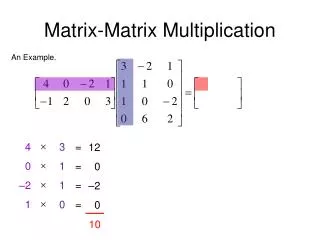
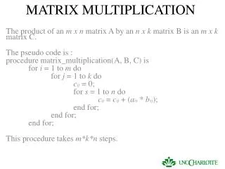
Multiplying Matrices • Two matrices, A with (p x q) matrix and B with (q x r) matrix, can be multiplied to get C with dimensions p x r, usingscalar multiplications
Ex2:Matrix-chain multiplication We are given a sequence (chain) <A1, A2, ..., An> of n matrices to be multiplied, and we wish to compute the product. A1.A2…An. Matrix multiplication is associative, and so all parenthesizations yield the same product, (A1 (A2 (A3 A4))) , (A1 ((A2 A3) A4)) , ((A1 A2) (A3 A4)) , ((A1 (A2 A3)) A4) , (((A1 A2) A3) A4).
Matrix-chain multiplication – cont. We can multiply two matrices A and B only if they are compatible the number of columns of A must equal the number of rows of B. If A is a p × q matrix and B is a q × r matrix, the resulting matrix C is a p × r matrix. The time to compute C is dominated by the number of scalar multiplications, which is p q r.
Matrix-chain multiplication – cont. • Ex: consider the problem of a chain <A1, A2, A3> of three matrices, with the dimensions of 10 × 100, 100 × 5, and 5 × 50, respectively. • If we multiply according to ((A1 A2) A3), we perform 10 · 100 · 5 = 5000 scalar multiplications to compute the 10 × 5 matrix product A1 A2, plus another 10 · 5 · 50 = 2500 scalar multiplications to multiply this matrix byA3 for a total of 7500 scalar multiplications • If instead , we multiply as (A1 (A2 A3)), we perform 100 · 5 · 50 = 25,000 scalar multiplications to compute the 100 × 50 matrix product A2 A3, plus another 10 · 100 · 50 = 50,000 scalar multiplications to multiply A1 by this matrix, for a total of 75,000 scalar multiplications. Thus, computing the product according to the first parenthesization is 10 times faster.
Matrix Chain Multiplication (MCM) Problem • Input: • Matrices A1, A2, …, An, each Ai of sizepi-1 x pi, • Output: • Fully parenthesised product A1 x A2 x … x An that minimizes the number of scalar multiplications. • Note: • In MCM problem, we are not actually multiplying matrices • Our goal is only to determine an order for multiplying matrices that has the lowest cost
Matrix Chain Multiplication (MCM) Problem • Typically, the time invested in determining this optimal order is more than paid for by the time saved later on when actually performing the matrix multiplications • So, exhaustively checking all possible parenthesizations does not yield an efficient algorithm
Counting the Number of Parenthesizations Denote the number of alternative parenthesizations of a sequence of (n) matrices by P(n) then a fully parenthesized matrix product is given by: If n = 4 <A1,A2,A3,A4> then the number of alternative parenthesis is =5 P(4) =P(1) P(4-1) + P(2) P(4-2) + P(3) P(4-3) = P(1) P(3) + P(2) P(2) + P(3) P(1)= 2+1+2=5 P(3) =P(1) P(2) + P(2) P(1) = 1+1=2 P(2) =P(1) P(1)= 1 (A1 (A2 (A3 A4))) , (A1 ((A2 A3) A4)) , ((A1 A2) (A3 A4)) , ((A1 (A2 A3)) A4) , (((A1 A2) A3) A4).
Step 2: Recursive Solution • Next we define the cost of optimal solution recursively in terms of the optimal solutions to sub-problems • For MCM, sub-problems are: • problems of determining the min-cost of a parenthesization of Ai Ai+1…Aj for 1 <= i <=j <=n • Let m[i, j] = min # of scalar multiplications needed to compute the matrix Ai...j. • For the whole problem, we need to find m[1, n]
Step 2: Recursive Solution • Since Ai..j can be obtained by breaking it into Ai..k Ak+1..j, We have (each Ai of size pi-1 x pi) • m[i, j] = m[i, k] + m[k+1, j] + pi-1pkpj • There are j-i possible values for k: i <= k <= j • Since the optimal parenthesization must use one of these values for k, we need only check them all to find the best.
Step 3: Computing the Optimal Costs The following code assumes that matrix Ai has dimensions pi-1 x pi for i =1,2, …, n
Step 4: Constructing an Optimal Solution • Although Matrix-Chain-Order determines the optimal numberof scalar multiplications needed to compute a matrix-chain product, it does not directly show how to multiply the matrices • Using table s, we can construct an optimal solution