Download
1 / 29
300 likes | 581 Views
Chapter 3 Some Special Distributions. Math 6203 Fall 2009 Instructor: Ayona Chatterjee. 3.1 The Binomial and Related Distributions. Bernoulli Distribution.

E N D
Chapter 3Some Special Distributions Math 6203 Fall 2009 Instructor: Ayona Chatterjee
Bernoulli Distribution • A Bernoulli experiment is a random experiment in which the outcome can be classified in one of two mutually exclusive and exhaustive ways. • Example: defective/non-defective, success/failure. • A sequence of independent Bernoulli trials has a fixed probability of success p.
Let X be a random variable associated with a Bernoulli trial. • X = 1 implies a success. • X = 0 implies a failure. • The pmf of X can be written as : • p(x)=px(1-p)1-x x=0,1 • In a sequence of n Bernoulli trials, we are often interested in a total of X number of successes.
Binomial Experiment • Independent and identical n trials. • Probability of success p is fixed for each trial. • Only two possible outcomes for each trial. • Number of trails are fixed.
Binomial Distribution • The random variable X which counts the number of success of a Binomial experiment is said to have a Binomial distribution with parameters n and p and its pmf is given by:
Negative Binomial Distribution • Consider a sequence of independent repetitions of a random experiment with constant probability p of success. Let the random variable Y denote the total number of failures in this sequence before the rth success that is, Y +r is equal to the number of trials required to produce exactly r successes. The pmf of Y is called a Negative Binomial distribution
Thus the probability of getting r-1 successes in the first y+r-1 trials and getting the rth success in the (y+r)thtrial gives the pmf of Y as
Geometric Distribution • The special case of r = 1 in the negative binomial, that is finding the first success in y trials gives the geometric distribution. • Thus we can re-write • P(Y)=p qy-1 for y = 1, 2, 3, …. • Lets find mean and variance for the Geometric Distribution.
Multinomial Distribution • Define the random variable Xi to be equal to the number of outcomes that are elements of Ci , i= 1, 2, … k-1. Here C1, C2, … Ck are k mutually exhaustive and exclusive outcomes of the experiment. The experiment is repeated n number of times. The multinomial distribution is
Trinomial Distribution • Let n= 3 in the multinomial distribution and we let X1 = X and X2= Y, then n –X-Y = X3 we have a trinomial distribution with the joint pmf of X and Y given as
3.2 The Poisson Distribution • A random variable that has a pmf of the form p(x) as given below is said to have a Poisson distribution with parameter m.
Poisson Postulates • Let g(x,w) denote the probability of x changes in each interval of length w. • Let the symbol o(h) represent any function such that • The postulates are • g(1,h)=λh+o(h), where λ is a positive constant and h > 0. • and • The number of changes in nonoverlapping intervals are independent.
Note • The number of changes in X in an interval of length w has a Poisson distribution with parameter m = wλ
3.3 The Gamma, Chi and Beta Distributions • The gamma function of α can be written as
The Gamma Distribution • A random variable X that has a pdf of the form below is said to have a gamma distribution with parameters α and β.
Exponential Distribution • The gamma distribution is used to model wait times. • W has a gamma distribution with α = k and β= 1/ λ. If W is the waiting time until the first change, that is k = 1, the pdf of W is the exponential distribution with parameter λ and its density is given as
Chi-Square Distribution • A special case of the Gamma distribution with α=r/2 and β=2 gives the Chi-Square distribution. Here r is a positive integer called the degrees of freedom.
Beta Distribution • A random variable X is said to have a beta distribution with parameters α and β if its density is given as follows
The Normal Distribution • We say a random variable X has a normal distribution if its pdf is given as below. The parameters μ and σ2 are the mean and variance of X respectively. We write X has N(μ,σ2).
The mgf • The moment generating function for X~N(μ,σ2) is
The t-distribution • Let W be a random variable with N(0,1) and let V denote a random variable with Chi-square distribution with r degrees of freedom. Then • Has a t-distribution with pdf
The F-distribution • Consider two independent chi-square variables each with degrees of freedom r1 and r2. • Let F = (U/r1)/(V/r2) • The variable F has a F-distribution with parameters r1 and r2 and its pdf is