Download
1 / 79
810 likes | 944 Views
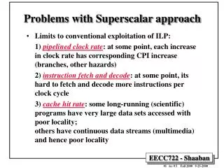
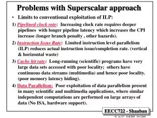
Problems with Superscalar approach. Limits to conventional exploitation of ILP: 1) Pipelined clock rate : Increasing clock rate requires deeper pipelines with longer pipeline latency which increases the CPI increase (longer branch penalty , other hazards).

E N D
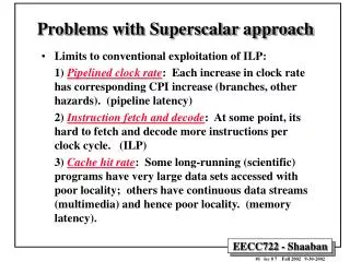
Problems with Superscalar approach • Limits to conventional exploitation of ILP: 1) Pipelined clock rate: Increasing clock rate requires deeper pipelines with longer pipeline latency which increases the CPI increase (longer branch penalty , other hazards). 2) Instruction Issue Rate: Limited instruction level parallelism (ILP) reduces actual instruction issue/completion rate. (vertical & horizontal waste) 3) Cache hit rate: Data-intensive scientific programs have very large data sets accessed with poor locality; others have continuous data streams (multimedia) and hence poor locality. (poor memory latency hiding). 4) Data Parallelism: Poor exploitation of data parallelism present in many scientific and multimedia applications, where similar independent computations are performed on large arrays of data (Limited ISA, hardware support). • As a result, actual achieved performance is much less than peak potential performance and low computational energy efficiency (computations/watt) Papers: VEC-1, VEC-2, VEC-3
X86 CPU Cache/Memory Performance Example:AMD Athlon T-Bird Vs. Intel PIII, Vs. P4 AMD Athlon T-Bird 1GHZ L1: 64K INST, 64K DATA (3 cycle latency), both 2-way L2: 256K 16-way 64 bit Latency: 7 cycles L1,L2 on-chip Data working set larger than L2 Intel P 4, 1.5 GHZ L1: 8K INST, 8K DATA (2 cycle latency) both 4-way 96KB Execution Trace Cache L2: 256K 8-way 256 bit , Latency: 7 cycles L1,L2 on-chip Intel PIII 1 GHZ L1: 16K INST, 16K DATA (3 cycle latency) both 4-way L2: 256K 8-way 256 bit , Latency: 7 cycles L1,L2 on-chip Impact of long memory latency for large data working sets Source: http://www1.anandtech.com/showdoc.html?i=1360&p=15 From 551
Flynn’s 1972 Classification of Computer Architecture • Single Instruction stream over a Single Data stream (SISD): Conventional sequential machines (Superscalar, VLIW). • Single Instruction stream over Multiple Data streams (SIMD): Vector computers, array of synchronized processing elements. (exploit data parallelism) • Multiple Instruction streams and a Single Data stream (MISD): Systolic arrays for pipelined execution. • Multiple Instruction streams over Multiple Data streams (MIMD): Parallel computers: • Shared memory multiprocessors (e.g. SMP, CMP, NUMA, SMT) • Multicomputers: Unshared distributed memory, message-passing used instead (Clusters) From 756 Lecture 1
Data Parallel Systems SIMD in Flynn taxonomy • Programming model: Data Parallel • Operations performed in parallel on each element of data structure • Logically single thread of control, performs sequential or parallel steps • Conceptually, a processor is associated with each data element • Architectural model • Array of many simple, cheap processors each with little memory • Processors don’t sequence through instructions • Attached to a control processor that issues instructions • Specialized and general communication, cheap global synchronization • Example machines: • Thinking Machines CM-1, CM-2 (and CM-5) • Maspar MP-1 and MP-2, From 756 Lecture 1
SCALAR (1 operation) VECTOR (N operations) v2 v1 r2 r1 + + r3 v3 vector length addv.d v3, v1, v2 Add.d F3, F1, F2 Alternative Model:Vector Processing • Vector processing exploits data parallelism by performing the same computations on linear arrays of numbers "vectors” using one instruction. The maximum number of elements in a vector is referred to as the Maximum Vector Length (MVL). Scalar ISA (RISC or CISC) Vector ISA Up to Maximum Vector Length (MVL) VEC-1 Typical MVL = 64 (Cray)
Vector Applications Applications with high degree of data parallelism (loop-level parallelism), thus suitable for vector processing. Not Limited to scientific computing • Astrophysics • Atmospheric and Ocean Modeling • Bioinformatics • Biomolecular simulation: Protein folding • Computational Chemistry • Computational Fluid Dynamics • Computational Physics • Computer vision and image understanding • Data Mining and Data-intensive Computing • Engineering analysis (CAD/CAM) • Global climate modeling and forecasting • Material Sciences • Military applications • Quantum chemistry • VLSI design • Multimedia Processing (compress., graphics, audio synth, image proc.) • Standard benchmark kernels (Matrix Multiply, FFT, Convolution, Sort) • Lossy Compression (JPEG, MPEG video and audio) • Lossless Compression (Zero removal, RLE, Differencing, LZW) • Cryptography (RSA, DES/IDEA, SHA/MD5) • Speech and handwriting recognition • Operating systems/Networking (memcpy, memset, parity, checksum) • Databases (hash/join, data mining, image/video serving) • Language run-time support (stdlib, garbage collection)
Increasing Instruction-Level Parallelism • A common way to increase parallelism among instructions is to exploit parallelism among iterations of a loop • (i.e Loop Level Parallelism, LLP). • This is accomplished by unrolling the loop either statically by the compiler, or dynamically by hardware, which increases the size of the basic block present. • In this loop every iteration can overlap with any other iteration. Overlap within each iteration is minimal. for (i=1; i<=1000; i=i+1;) x[i] = x[i] + y[i]; • In vector machines, utilizing vector instructions is an important alternative to exploit loop-level parallelism, • Vector instructions operate on a number of data items. The above loop would require just four such instructions if vector length = 1000 is supported. Vector Code Scalar Code Load_vector V1, Rx Load_vector V2, Ry Add_vector V3, V1, V2 Store_vector V3, Rx From 551
Loop-Level Parallelism (LLP) Analysis • LLP analysis is normally done at the source level or close to it since assembly language and target machine code generation introduces a loop-carried dependence, in the registers used for addressing and incrementing. • Instruction level parallelism (ILP) analysis is usually done when instructions are generated by the compiler. • Analysis focuses on whether data accesses in later iterations are data dependent on data values produced in earlier iterations. e.g. in for (i=1; i<=1000; i++) x[i] = x[i] + s; the computation in each iteration is independent of the previous iterations and the loop is thus parallel. The use of X[i] twice is within a single iteration. From 551
LLP Analysis Examples • In the loop: for (i=1; i<=100; i=i+1) { A[i+1] = A[i] + C[i]; /* S1 */ B[i+1] = B[i] + A[i+1];} /* S2 */ } • S1 uses a value computed in an earlier iteration, since iteration i computes A[i+1] read in iteration i+1 (loop-carried dependence, prevents parallelism). • S2 uses the value A[i+1], computed by S1 in the same iteration (not loop-carried dependence). From 551
LLP Analysis Examples • In the loop: for (i=1; i<=100; i=i+1) { A[i] = A[i] + B[i]; /* S1 */ B[i+1] = C[i] + D[i]; /* S2 */ } • S1 uses a value computed by S2 in a previous iteration (loop-carried dependence) • This dependence is not circular (neither statement depend on itself; S1 depends on S2 but S2 does not depend on S1. • Can be made parallel by replacing the code with the following: A[1] = A[1] + B[1]; for (i=1; ii<=99; i=i+1) { B[i+1] = C[i] + D[i]; A[i+1] = A[i+1] + B[i+1]; } B[101] = C[100] + D[100]; Scalar code Vectorizable code Scalar code From 551
A[1] = A[1] + B[1]; B[2] = C[1] + D[1]; A[99] = A[99] + B[99]; B[100] = C[99] + D[99]; A[2] = A[2] + B[2]; B[3] = C[2] + D[2]; A[100] = A[100] + B[100]; B[101] = C[100] + D[100]; LLP Analysis Example for (i=1; i<=100; i=i+1) { A[i] = A[i] + B[i]; /* S1 */ B[i+1] = C[i] + D[i]; /* S2 */ } Original Loop: Iteration 99 Iteration 100 Iteration 1 Iteration 2 . . . . . . . . . . . . Loop-carried Dependence • A[1] = A[1] + B[1]; • for (i=1; i<=99; i=i+1) { • B[i+1] = C[i] + D[i]; • A[i+1] = A[i+1] + B[i+1]; • } • B[101] = C[100] + D[100]; Modified Parallel Loop: Iteration 98 Iteration 99 . . . . Iteration 1 Loop Start-up code A[1] = A[1] + B[1]; B[2] = C[1] + D[1]; A[99] = A[99] + B[99]; B[100] = C[99] + D[99]; A[2] = A[2] + B[2]; B[3] = C[2] + D[2]; A[100] = A[100] + B[100]; B[101] = C[100] + D[100]; Not Loop Carried Dependence Loop Completion code From 551
Vector vs. Single-issue Scalar Vector • One instruction fetch,decode, dispatch per vector • Structured register accesses • Smaller code for high performance, less power in instruction cache misses • Bypass cache (for data) • One TLB lookup pergroup of loads or stores • Move only necessary dataacross chip boundary • Single-issue Scalar • One instruction fetch, decode, dispatch per operation • Arbitrary register accesses,adds area and power • Loop unrolling and software pipelining for high performance increases instruction cache footprint • All data passes through cache; waste power if no temporal locality • One TLB lookup per load or store • Off-chip access in whole cache lines
Vector vs. Superscalar Vector • Control logic growslinearly with issue width • Vector unit switchesoff when not in use- higher energy efficiency • Vector instructions expose data parallelism without speculation • Software control ofspeculation when desired: • Whether to use vector mask or compress/expand for conditionals • Superscalar • Control logic grows quad-ratically with issue width • Control logic consumes energy regardless of available parallelism • Speculation to increase visible parallelism wastes energy and adds complexity
Properties of Vector Processors • Each result in a vector operation is independent of previous results (Loop Level Parallelism, LLP exploited)=> long pipelines used, compiler ensures no dependencies=> higher clock rate (less complexity) • Vector instructions access memory with known patterns=> Highly interleaved memory with multiple banks used to provide the high bandwidth needed and hide memory latency.=> Amortize memory latency of over many vector elements=> no (data) caches usually used. (Do use instruction cache) • A single vector instruction implies a large number of computations (replacing loops or reducing number of iterations needed)=> Fewer instructions fetched/executed => Reduces branches and branch problems in pipelines
Changes to Scalar Processor to Run Vector Instructions • A vector processor typically consists of an ordinary pipelined scalar unit plus a vector unit. • The scalar unit is basically not different than advanced pipelined CPUs, commercial vector machines have included both out-of-order scalar units (NEC SX/5) and VLIW scalar units (Fujitsu VPP5000). • Computations that don’t run in vector mode don’t have high ILP, so can make scalar CPU simple. • The vector unit supports a vector ISA including decoding of vector instructions which includes: • Vector functional units. • ISA vector register bank, vector control registers (vector length, mask) • Vector memory Load-Store Units (LSUs). • Multi-banked main memory • Send scalar registers to vector unit (for vector-scalar ops). • Synchronization for results back from vector register, including exceptions.
Basic Types of Vector Architecture • Types of architecture/ISA for vector processors: • Memory-memory vector processors: all vector operations are memory to memory • Vector-register processors: all vector operations between vector registers (except load and store) • Vector equivalent of load-store scalar architectures • Includes all vector machines since the late 1980 Cray, Convex, Fujitsu, Hitachi, NEC • We assume vector-register for rest of the lecture
Basic Structure of Vector Register Architecture Multi-Banked memory for bandwidth and latency-hiding Pipelined Vector Functional Units Vector Load-Store Units (LSUs) MVL elements Vector Control Registers VLR Vector Length Register VM Vector Mask Register VEC-1
Components of Vector Processor • Vector Register: fixed length bank holding a single vector • has at least 2 read and 1 write ports • typically 8-32 vector registers, each holding MVL = 64-128 64-bit elements • Vector Functional Units (FUs): fully pipelined, start new operation every clock • typically 4 to 8 FUs: FP add, FP mult, FP reciprocal (1/X), integer add, logical, shift; may have multiple of same unit • Vector Load-Store Units (LSUs): fully pipelined unit to load or store a vector; may have multiple LSUs • Scalar registers: single element for FP scalar or address • System Interconnects: Cross-bar to connect FUs , LSUs, registers VEC-1
Vector ISA Issues: How To Pick Maximum Vector Length (MVL)? • Longer good because: 1) Hide vector startup time 2) Lower instruction bandwidth 3) Tiled access to memory reduce scalar processor memory bandwidth needs 4) If known maximum length of app. is < MVL, no strip mining (vector loop) overhead is needed. 5) Better spatial locality for memory access • Longer not much help because: 1) Diminishing returns on overhead savings as keep doubling number of elements. 2) Need natural application vector length to match physical vector register length, or no help VEC-1
Vector Implementation • Vector register file: • Each register is an array of elements • Size of each register determines maximumvector length (MVL) supported. • Vector Length Register (VLR) determines vector length for a particular vector operation • Vector Mask Register (VM) determines which elements of a vector will be computed • Multiple parallel execution units = “lanes”(sometimes called “pipelines” or “pipes”) • Multiples pipelined functional units are each assigned a number of computations of a single vector instruction.
Using multiple Functional Units to Improve the Performance of a A single Vector Add Instruction (a) has a single add pipeline and can complete one addition per cycle. The machine shown in (b) has four add pipelines and can complete four additions per cycle. One Lane Four Lanes MVL lanes? Data parallel system, SIMD array?
The VMIPS Vector FP Instructions Vector FP Vector Memory Vector Index Vector Mask Vector Length VEC-1
Vector Memory operations • Load/store operations move groups of data between registers and memory • Three types of addressing: • Unit stride Fastest memory access LV (Load Vector), SV (Store Vector): LV V1, R1 Load vector register V1 from memory starting at address R1 SV R1, V1 Store vector register V1 into memory starting at address R1. • Non-unit(constant) stride LVWS (Load Vector With Stride), SVWS (Store Vector With Stride): LVWS V1,(R1,R2) Load V1 from address at R1 with stride in R2, i.e., R1+i × R2. SVWS (R1,R2),V1 Store V1 from address at R1 with stride in R2, i.e., R1+i × R2. • Indexed (gather-scatter) • Vector equivalent of register indirect • Good for sparse arrays of data • Increases number of programs that vectorize LVI (Load Vector Indexed or Gather), SVI (Store Vector Indexed or Scatter): LVI V1,(R1+V2) Load V1 with vector whose elements are at R1+V2(i), i.e., V2 is an index. SVI (R1+V2),V1 Store V1 to vector whose elements are at R1+V2(i), i.e., V2 is an index. (i size of element) VEC-1
DAXPY (Y = a*X + Y) Assuming vectors X, Y are length 64 =MVL Scalar vs. Vector L.D F0,a ;load scalar a LV V1,Rx ;load vector X MULVS.D V2,V1,F0 ;vector-scalar mult. LV V3,Ry ;load vector Y ADDV.D V4,V2,V3 ;add SV Ry,V4 ;store the result L.D F0,a DADDIU R4,Rx,#512 ;last address to load loop: L.D F2, 0(Rx) ;load X(i) MUL.D F2,F0,F2 ;a*X(i) L.D F4, 0(Ry) ;load Y(i) ADD.D F4,F2, F4 ;a*X(i) + Y(i) S.D F4,0(Ry) ;store into Y(i) DADDIU Rx,Rx,#8 ;increment index to X DADDIU Ry,Ry,#8 ;increment index to Y DSUBU R20,R4,Rx ;compute bound BNEZ R20,loop ;check if done VLR = 64 VM = (1,1,1,1 ..1) 578 (2+9*64) vs. 321 (1+5*64) ops (1.8X) 578 (2+9*64) vs. 6 instructions (96X) 64 operation vectors + no loop overhead also 64X fewer pipeline hazards
1: LV V1,Rx ;load vector X 2: MULV V2,F0,V1 ;vector-scalar mult. LV V3,Ry ;load vector Y 3: ADDV V4,V2,V3 ;add 4: SV Ry,V4 ;store the result Vector Execution Time • Time = f(vector length, data dependicies, struct. Hazards, C) • Initiation rate: rate that FU consumes vector elements.(= number of lanes; usually 1 or 2 on Cray T-90) • Convoy: set of vector instructions that can begin execution in same clock (no struct. or data hazards) • Chime: approx. time for a vector element operation (~ one clock cycle). • m convoys take m chimes; if each vector length is n, then they take approx. m x n clock cycles (ignores overhead; good approximation for long vectors) Assuming one lane is used 4 conveys, 1 lane, VL=64 => 4 x 64 = 256 cycles (or 4 cycles per result vector element) VEC-1
Vector FU Start-up Time • Start-up time: pipeline latency time (depth of FU pipeline); another sources of overhead • Operation Start-up penalty (from CRAY-1) • Vector load/store 12 • Vector multiply 7 • Vector add 6 Assume convoys don't overlap; vector length = n: Convoy Start 1st result last result 1. LV 0 12 11+n (12+n-1) 2. MULV, LV 12+n 12+n+12 23+2n Load start-up 3. ADDV 24+2n 24+2n+6 29+3n Wait convoy 2 4. SV 30+3n 30+3n+12 41+4n Wait convoy 3 Start-up cycles VEC-1
Vector Load/Store Units & Memories • Start-up overheads usually longer for LSUs • Memory system must sustain (# lanes x word) /clock cycle • Many Vector Procs. use banks (vs. simple interleaving): 1) support multiple loads/stores per cycle => multiple banks & address banks independently 2) support non-sequential accesses (non unit stride) • Note: No. memory banks > memory latency to avoid stalls • m banks => m words per memory lantecy l clocks • if m < l, then gap in memory pipeline: clock: 0 … l l+1 l+2 … l+m- 1 l+m … 2 l word: -- … 0 1 2 … m-1 -- … m • may have 1024 banks in SRAM
Vector Memory Requirements Example • The Cray T90 has a CPU clock cycle of 2.167 ns (460 MHz) and in its largest configuration (Cray T932) has 32 processors each capable of generating four loads and two stores per CPU clock cycle. • The CPU clock cycle is 2.167 ns, while the cycle time of the SRAMs used in the memory system is 15 ns. • Calculate the minimum number of memory banks required to allow all CPUs to run at full memory bandwidth. • Answer: • The maximum number of memory references each cycle is 192 (32 CPUs times 6 references per CPU). • Each SRAM bank is busy for 15/2.167 = 6.92 clock cycles, which we round up to 7 CPU clock cycles. Therefore we require a minimum of 192 × 7 = 1344 memory banks! • The Cray T932 actually has 1024 memory banks, and so the early models could not sustain full bandwidth to all CPUs simultaneously. A subsequent memory upgrade replaced the 15 ns asynchronous SRAMs with pipelined synchronous SRAMs that more than halved the memory cycle time, thereby providing sufficient bandwidth/latency.
Vector Memory Access Example • Suppose we want to fetch a vector of 64 elements (each element 8 bytes) starting at byte address 136, and a memory access takes 6 clocks. How many memory banks must we have to support one fetch per clock cycle? With what addresses are the banks accessed? • When will the various elements arrive at the CPU? • Answer • Six clocks per access require at least six banks, but because we want the number of banks to be a power of two, we choose to have eight banks as shown on next slide
Vector Length Needed Not Equal to MVL • What to do when vector length is not exactly 64? • vector-length register (VLR) controls the length of any vector operation, including a vector load or store. (cannot be > MVL = the length of vector registers) do 10 i = 1, n 10 Y(i) = a * X(i) + Y(i) • Don't know n until runtime! n > Max. Vector Length (MVL)? • Vector Loop (Strip Mining) Vector length = n
Strip Mining • Suppose Vector Length > Max. Vector Length (MVL)? • Strip mining: generation of code such that each vector operation is done for a size Š to the MVL • 1st loop do short piece (n mod MVL), reset VL = MVL low = 1 VL = (n mod MVL) /*find the odd size piece*/ do 1 j = 0,(n / MVL) /*outer loop*/ do 10 i = low,low+VL-1 /*runs for length VL*/ Y(i) = a*X(i) + Y(i) /*main operation*/10 continue low = low+VL /*start of next vector*/ VL = MVL /*reset the length to max*/1 continue Time for loop: Vector loop iterations needed
Strip Mining 0 1st iteration n MOD MVL elements (odd size piece) For First Iteration (shorter vector) Set VL = n MOD MVL 0 < size < MVL VL -1 For MVL = 64 VL = 1 - 63 2nd iteration MVL elements For second Iteration onwards Set VL = MVL MVL (e.g. VL = MVL = 64) 3rd iteration MVL elements ì n/MVLù vector loop iterations needed MVL :: ::
Strip Mining Example • What is the execution time on VMIPS for the vector operation A = B × s, where s is a scalar and the length of the vectors A and B is 200 (MVL supported =64)? Answer • Assume the addresses of A and B are initially in Ra and Rb, s is in Fs, and recall that for MIPS (and VMIPS) R0 always holds 0. • Since (200 mod 64) = 8, the first iteration of the strip-mined loop will execute for a vector length of VL = 8 elements, and the following iterations will execute for a vector length = MVL = 64 elements. • The starting byte addresses of the next segment of each vector is eight times the vector length. Since the vector length is either 8 or 64, we increment the address registers by 8 × 8 = 64 after the first segment and 8 × 64 = 512 for later segments. • The total number of bytes in the vector is 8 × 200 = 1600, and we test for completion by comparing the address of the next vector segment to the initial address plus 1600. • Here is the actual code follows:
Strip Mining Example VLR = n MOD 64 = 200 MOD 64 = 8 For first iteration only VLR = MVL= 64 for second iteration onwards MTC1 VLR,R1 Move contents of R1 to the vector-length register. 4 vector loop iterations
Strip Mining Example 4 iterations Tloop = loop overhead = 15 cycles VEC-1
Strip Mining Example The total execution time per element and the total overhead time per element versus the vector length for the strip mining example MVL supported = 64
Vector Stride • Suppose adjacent vector elements not sequential in memory do 10 i = 1,100 do 10 j = 1,100 A(i,j) = 0.0 do 10 k = 1,100 10 A(i,j) = A(i,j)+B(i,k)*C(k,j) • Either B or C accesses not adjacent (800 bytes between) • stride: distance separating elements that are to be merged into a single vector (caches do unit stride) => LVWS (load vector with stride) instruction LVWS V1,(R1,R2) Load V1 from address at R1 with stride in R2, i.e., R1+i × R2. => SVWS (store vector with stride) instruction SVWS (R1,R2),V1 Store V1 from address at R1 with stride in R2, i.e., R1+i × R2. • Strides => can cause bank conflicts and stalls may occur.
Vector Stride Memory Access Example • Suppose we have 8 memory banks with a bank busy time of 6 clocks and a total memory latency of 12 cycles. How long will it take to complete a 64-element vector load with a stride of 1? With a stride of 32? Answer • Since the number of banks is larger than the bank busy time, for a stride of 1, the load will take 12 + 64 = 76 clock cycles, or 1.2 clocks per element. • The worst possible stride is a value that is a multiple of the number of memory banks, as in this case with a stride of 32 and 8 memory banks. • Every access to memory (after the first one) will collide with the previous access and will have to wait for the 6-clock-cycle bank busy time. • The total time will be 12 + 1 + 6 * 63 = 391 clock cycles, or 6.1 clocks per element.
Vector Chaining • Suppose: MULV.D V1,V2,V3 ADDV.D V4,V1,V5 ; separate convoys? • chaining: vector register (V1) is not treated as a single entity but as a group of individual registers, then pipeline forwarding can work on individual elements of a vector • Flexible chaining: allow vector to chain to any other active vector operation => more read/write ports • As long as enough HW is available , increases convoy size • With chaining, the above sequence is treated as a single convoy and the total running time becomes: Vector length + Start-up timeADDV + Start-up timeMULV
Vector Chaining Example • Timings for a sequence of dependent vector operations MULV.D V1,V2,V3 ADDV.D V4,V1,V5 both unchained and chained. m convoys with n elements take: startup + m x n cycles Here startup = 7 + 6 = 13 cycles n = 64 = 7 + 64 + 6 + 64 = startup + m x n = 13 + 2 x 64 Two Convoys m =2 One Convoy m =1 = 7 + 6 + 64 = startup + m x n = 13 + 1 x 64 141 / 77 = 1.83 times faster with chaining VEC-1
Vector Conditional Execution • Suppose: do 100 i = 1, 64 if (A(i) .ne. 0) then A(i) = A(i) – B(i) endif 100 continue • vector-mask controltakes a Boolean vector: when vector-mask (VM) registeris loaded from vector test, vector instructions operate only on vector elements whose corresponding entries in the vector-mask register are 1. • Still requires a clock cycle per element even if result not stored.
Vector Conditional Execution Example Compare the elements (EQ, NE, GT, LT, GE, LE) in V1 and V2. If condition is true, put a 1 in the corresponding bit vector; otherwise put 0. Put resulting bit vector in vector mask register (VM). The instruction S--VS.D performs the same compare but using a scalar value as one operand. S--V.D V1, V2 S--VS.D V1, F0 LV, SV Load/Store vector with stride 1
Vector operations: Gather, Scatter • Suppose: do 100 i = 1,n 100 A(K(i)) = A(K(i)) + C(M(i)) • gather (LVI,load vector indexed), operation takes an index vectorand fetches the vector whose elements are at the addresses given by adding a base address to the offsets given in the index vector => a nonsparse vector in a vector register LVI V1,(R1+V2) Load V1 with vector whose elements are at R1+V2(i), i.e., V2 is an index. • After these elements are operated on in dense form, the sparse vector can be stored in expanded form by a scatter store (SVI, store vector indexed), using the same or different index vector SVI (R1+V2),V1 Store V1 to vector whose elements are at R1+V2(i), i.e., V2 is an index. • Can't be done by compiler since can't know K(i), M(i) elements • Use CVI (create vector index)to create index 0, 1xm, 2xm, ..., 63xm
Gather, Scatter Example Assuming that Ra, Rc, Rk, and Rm contain the starting addresses of the vectors in the previous sequence, the inner loop of the sequence can be coded with vector instructions such as: (index vector) (index vector) LVI V1, (R1+V2) (Gather) Load V1 with vector whose elements are at R1+V2(i), i.e., V2 is an index. SVI (R1+V2), V1 (Scatter) Store V1 to vector whose elements are at R1+V2(i), i.e., V2 is an index. Index vectors Vk Vm already initialized
Vector Conditional Execution Using Gather, Scatter • The indexed loads-stores and the create an index vector CVI instruction provide an alternative method to support conditional vector execution. CVI V1,R1 Create an index vector by storing the values 0, 1 × R1, 2 × R1,...,63 × R1 into V1. V2 Index Vector VM Vector Mask VEC-1
Vector Example with dependencyMatrix Multiplication /* Multiply a[m][k] * b[k][n] to get c[m][n] */ for (i=1; i<m; i++) { for (j=1; j<n; j++) { sum = 0; for (t=1; t<k; t++) { sum += a[i][t] * b[t][j]; } c[i][j] = sum; } } C mxn = A mxk X B kxn Dot product
Scalar Matrix Multiplication /* Multiply a[m][k] * b[k][n] to get c[m][n] */ for (i=1; i<m; i++) { for (j=1; j<n; j++) { sum = 0; for (t=1; t<k; t++) { sum += a[i][t] * b[t][j]; } c[i][j] = sum; } } Inner loop t = 1 to k (vector dot product loop) (for a given i, j produces one element C(i, j) k n n i j t m X = t C(i, j) k n A(m, k) B(k, n) C(m, n) Second loop j = 1 to n Outer loop i = 1 to m For one iteration of outer loop (on i) and second loop (on j) inner loop (t = 1 to k) produces one element of C, C(i, j) Inner loop (one element of C, C(i, j) produced) Vectorize inner t loop?