Download
1 / 52
520 likes | 744 Views
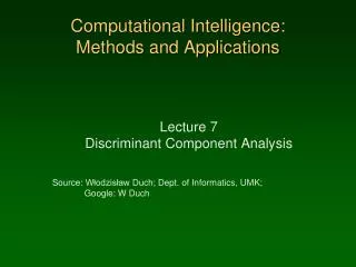
Lecture 7 Discriminant Component Analysis Source: Włodzisław Duch ; Dept. of Informatics, UMK ; Google: W Duch. Computational Intelligence: Methods and Applications. PCA problem. PCA transformation for 2D data:.

E N D
Lecture 7Discriminant Component Analysis Source: Włodzisław Duch; Dept. of Informatics,UMK; Google: W Duch Computational Intelligence: Methods and Applications
PCA problem PCA transformation for 2D data: PCA give worst possible solution here from the point of view of seeing the structure of the data. PCA is completely unsupervised, knows only about variance, but nothing about different classes of data. Goal: find direction of projection that shows more structure in the data, using class structure; this will then be supervised approach. “Discriminant coordinates” should reveal class structure much better.
PCA does not find the best combination to reveal the structure of data. No information about data structure, class labels, is used in PCA. If class info is available (or clusterization has been performed): find mean vectors, find projection direction that maximizes separation of means for 2 classes: B Maximize separation Bdirection ||B||=1 defines line passing through 0, the value of projection Y=BTX If data clusters are spherical or Gaussian B is a good choice; find more projection directions Biin the space orthogonal to B1=B. Here direction X2 is a better choice!
If one interesting direction B1 has been found in the n-vector X=[X(1),X(2)...X(n)] data space, each with d dimensions X(1)=(X1 ... Xd) then orthogonal space is created using projection operator: Reminder: orthogonal projection Here P1 is a dxd matrix that applied to X rotates the data space leaving only components that are orthogonal to B1(normalized vector, ||B1||=1). if B2is orthogonal to B1 Create X’ = P1 X and repeat the same procedure to find an interesting orthogonal vector B2. Projection operator orthogonalizing to the [B1,B2] space is simply P2 = I-B1B1T-B2B2T, adding more terms for higher Pn.
This is not an optimal solution, although it is better than PCA ... Covariance of the two distributions should be taken into account: Greater separation Figure from: Chapter 4, Elements of statistical learning. By Hasti, Tibshirani and Friedman 2001
Find transformation Y = WT·X, that maximizes the distance of projected mean values: Within-class scatter But scaling W may create arbitrarily large differences! This distance should be large relatively to the variance (scatter): Within-class scatter, or variance without normalization constant 1/(n-1). i=1,2class of vectors, j=1..n(Ci)sample Total within-class scatter; variances could be also used.
Maximize the Fisher criterion function: Fisher criterion This is maximum for large separation and small within-class variance. It does not depend on the norm of W, only on the direction. Skis the within-class scatter matrix for class Ck.
Total within-class scatter matrix SI = S1+S2 The difference of the means may be written as: Fisher linear discriminant SBis the between-class scatter matrix. Fisher criterion is: This is a Rayleigh quotient, and the solution to this maximization problem is quite simple using variational techniques. This procedure defines FDA = Fisher Discriminant Analysis.
Small perturbation of W around maximum should not influence J(W), therefore the two scalars below should be proportional: FDA solution This is generalized eigenvalue equation, but since SImay be inverted: it becomes standard eigenvalue problem. First direction is found from: because only the direction of W, not the length, is important, and a(W) is a scalar that does not change direction. More directions are found from the eigenequation or repeating the procedure in subspace orthogonal to W.
FDA is frequently used for classification, projecting data on a line. For visualization generating the second FDA vector in a two-class problem is not so trivial. This is due to the fact that the rank of the SB matrix for the 2-class problems is 1 (why?), or for the K class problems it is K-1. Also SI may be ill-conditioned. FDA second vector Solutions: pseudoinverse for SImakes it more stable; perturbations of the SI values may help. Please consult A. Webb, Statistical pattern analysis, Chapter 4.3.3 for detailed discussion of numerical problems. Example: FDA projections of hypercubes (using Matlab).
Example: Matlab PCA solution for projections of hypercubes. For 3D cube taking all 8 vertices, from (0,0,0) to (1,1,1): PCA selects one of the walls. PCA for 3D cube Removing (0,0,0) and using only 7 vertices better structure is shown.
For 4D cube taking 15 vertices, from (0,0,0,1) to (1,1,1,1): For 5D cube taking 31 vertices, from (0,0,0,0,1) to (1,1,1,1,1): PCA for 4/5D hypercube
FDA requires classes: here odd/even parity of vertex bit strings. Left: pseudoinverse SI , right – perturbed SB matrix FDA for 3D cube
With perturbed SB matrix: note that vertices from the same class (same parity) are projected on a vertical line; perturbation does not make them uniformly spaced along this line. FDA for 4/5D cube
For normalized data Xi [0,1] FDA projection is close to the lattice projection, defined as W1=[1,1,..1] direction and W2 maximizing separation of the points with fixed number of 1 bits. Lattice projection Lattice projections may be quite useful up to 6 dimensions.
The state of a dynamical X(t) system in 4 dimensions changes in time. Where are the attractors and what is this system doing? Dynamical lattice projection Seems to be going between 1000 and 0100 and 1100. Second system presented in 2 PCA coordinates has initially 4 attractors but becomes finally chaotic.
11 vowels were segmented from speech of a number of people, and 10 features were derived for each vowel. Examples of 2D scatterograms for standardized data are below. Vowel example
PCA components 1-2, 1-3 i 2-3 Vowel PCA
FDA components 1-2 Vowel FDA Figure from: Chapter 4, Elements of statistical learning. By Hasti, Tibshirani and Friedman 2001
Figure from: Chapter 4, Elements of statistical learning. By Hasti, Tibshirani and Friedman 2001 FDA higher components
Figure from: Chapter 4, Elements of statistical learning. By Hasti, Tibshirani and Friedman 2001 FDA prototypes
Computational Intelligence: Methods and Applications Lecture 8 Projection Pursuit &Independent Component Analysis Source: Włodzisław Duch; Dept. of Informatics,UMK; Google: W Duch
Exploratory Projection Pursuit (PP) PCA and FDA are linear, PP may be linear or non-linear. Find interesting “criterion of fit”, or “figure of merit” function, that allows for low-dim (usually 2D or 3D) projection. General transformation with parameters W. Index of “interestingness” Interesting indices may use a priori knowledge about the problem: 1. mean nearest neighbor distance – increase clustering of Y(j)2. maximize mutual information between classes and features 3. find projection that have non-Gaussian distributions. The last index does not use a priori knowledge; it leads to the Independent Component Analysis (ICA), unsupervised method.ICA features are not only uncorrelated, but also independent.
Kurtosis ICA is a special version of PP, recently very popular. Gaussian distributions of variable Y are characterized by 2 parameters: mean value: variance: These are the first 2 moments of distribution; all higher are 0 for G(Y). One simple measure of non-Gaussianity of projections is the 4-th moment (cumulant) of the distribution, called kurtosis, measures “concentration” of the distribution. It the mean E{Y}=0 kurtosis is: Super-Gaussian distribution: long tail, peak at zero, k4(Y)>0, like binary image data. sub-Gaussian distribution is more flat and has k4(Y)<0, like speech signal data. Find interesting direction looking for maxW |k4(Y(W))|
Correlation and independence Features Yi, Yjare uncorrelated if covariance is diagonal, or: Variables Yi are statistically independent if their joint probability distribution is a product of probabilities for all variables: Uncorrelated features are orthogonal, but may have higher-order dependencies, while any functions of independent features Yi, Yj This is much stronger condition than correlation; in particular the functions may be powers of variables; any non-Gaussian distribution after PCA transformation will still have some feature dependencies.
PP/ICA example Example: PCA and PP based on maximal kurtosis: note nice separation of the blue class.
Some remarks • Many algorithms for exploratory PP and ICA methods exist. • PP is used for visualization, dimensionality reduction & regression. • Nonlinear projections are frequently considered, but solutions are more numerically intensive. • PCA may also be viewed as PP, maximizing (for standard. data): Index I(Y;W) is based here on maximum variance. Other components are found in the space orthogonal to W1 Same index is used, with projection on space orthogonal to k-1PCs. PP/ICA description: Chap. 14.6, Friedman, Hastie, Tibshirani.
ICA demos • ICA has many applications in signal and image analysis. • Finding independent signal sources allows for separation of signals from different sources, removal of noise or artifacts. • Observations X are a linear mixture W of unknown sources Y Both W and Y are unknown! This is a blind separation problem. How can they be found? If Y are Independent Components and W linear mixing the problem is similar to PCA, only the criterion function is different. Play with ICA-Lab PCA/ICA Matlab software for signal/image analysis:http://www.bsp.brain.riken.go.jp/page7.html
ICA examples • Mixing simple signals: sinus + chainsaw. • Vectors X = samples of signals in some time window From: Chap. 14.6, Friedman, Hastie, Tibshirani: The elements of statistical learning.
ICA demo: images & audio • Play with ICA-Lab PCA/ICA Matlab software for signal/image analysis • from Cichocki’s lab, • http://www.bsp.brain.riken.go.jp/page7.html • X space for images: • take intensity of all pixels one vector per image, or • take smaller patches (ex: 64x64), increasing # vectors • 5 images: originals, mixed, convergence of ICA iterations • X space for signals: • sample the signal for some time Dt • 10 songs: mixed samples and separated samples • Good survey paper on ICA is at: http://www.cis.hut.fi/aapo/papers/NCS99web/
Further reading Many other visualization and dimensionality reduction methods exit. See the links here: http://www.is.umk.pl/~duch/CI.html#vis http://www.is.umk.pl /software.html#Visual Principal curves Web page http://www.iro.umontreal.ca/~kegl/research/pcurves/ Good page with research papers on manifold learning: http://www.cse.msu.edu/~lawhiu/manifold/ A. Webb, Chapter 6.3 on projection pursuit, chap. 9.3 on PCA Duda/Hart/Stork, chap. 3.8 on PCA and FDA Now we shall turn to non-linear methods inspired by the approach that is used by our brains.
Self-organization PCA, FDA, ICA, PP are all inspired by statistics, although some neural-inspired methods have been proposed to find interesting solutions, especially for non-linear PP versions. Brains learn to discover the structure of signals: visual, tactile, olfactory, auditory (speech and sounds). This is a good example of unsupervised learning: spontaneous development of feature detectors, compressing internal information that is needed to model environmental states (inputs). Some simple stimuli lead to complex behavioral patterns in animals; brains use specialized microcircuits to derive vital information from signals – for example, amygdala nuclei in rats sensitive to ultrasound signals signifying “cat around”.
Models of self-organizaiton SOM or SOFM (Self-Organized Feature Mapping) – self-organizing feature map, one of the simplest models. How can such maps develop spontaneously? Local neural connections: neuronsinteract strongly with those nearby, but weakly with those that are far (in addition inhibiting some intermediate neurons). History: von der Malsburg and Willshaw (1976), competitive learning, Hebb mechanisms, „Mexican hat” interactions, models of visual systems. Amari (1980) – models of continuous neural tissue. Kohonen (1981) - simplification, no inhibition; leaving two essential factors: competition and cooperation.
Computational Intelligence: Methods and Applications Lecture 9 Self-Organized Mappings Source: Włodzisław Duch; Dept. of Informatics,UMK; Google: W Duch
Brain maps • Tactile, motor, and olfactory data are most basic. • Such data is analyzed by animal brains using topographical organization of the brain cortex. • Somatosensory maps for tactile, temperature, pain, itching, and vibration signals. • Motor maps in frontal neocortex and cerebellum cortex. • Auditory tonotopic maps in temporal cortex. • Visual orientation maps in primary visual cortex. • Multimodal orientation maps (superior colliculus)
Senso-motoric map Visual signals are analyzed by maps coupled with motor maps and providing senso-motoric responses. Figure from: P.S. Churchland, T.J. Sejnowski, The computational brain. MIT Press, 1992
Representation of fingers Before Afterstimulation stimulation Hand Face
Models of self-organization SOM or SOFM (Self-Organized Feature Mapping) – self-organizing feature map, one of the simplest models. How can such maps develop spontaneously? Local neural connections: neuronsinteract strongly with those nearby, but weakly with those that are far (in addition inhibiting some intermediate neurons). History: von der Malsburg and Willshaw (1976), competitive learning, Hebb mechanisms, „Mexican hat” interactions, models of visual systems. Amari (1980) – models of continuous neural tissue. Kohonen (1981) - simplification, no inhibition; leaving two essential factors: competition and cooperation.
Self-Organized Map: idea Data: vectors XT = (X1, ... Xd) from d-dimensional space. Grid of nodes, with local processor (called neuron) in each node. Local processor # j has d adaptive parameters W(j). Goal: change W(j) parameters to recover data clusters in X space.
SOM algorithm: competition Nodes should calculate similarity of input data to their parameters. Input vectorXis compared to node parametersW. Similar = minimal distance or maximal scalar product. Competition: find node j=c with W most similar to X. Node number c is most similar to the input vectorX It is a winner, and it will learn to be more similar to X, hence this is a “competitive learning” procedure. Brain: those neurons that react to some signals pick it up and learn.
SOM algorithm: cooperation Cooperation: nodes on a grid close to the winnercshould behave similarly. Define the “neighborhoodfunction” O(c): t – iteration number (or time); rc – position of the winning node c (in physical space, usually 2D). ||r-rc||– distance from the winning node, scaled by sc(t). h0(t)– slowly decreasing multiplicative factor The neighborhood function determines how strongly the parameters of the winning node and nodes in its neighborhood will be changed, making them more similar to data X
SOM algorithm: dynamics Adaptation rule: take the winner nodec, and those in its neighborhood O(rc), change their parameters making them more similar to the data X • Select randomly new sample vector X, and repeat. • Decrease h0(t)slowly until there will be no changes. • Result: • W(i)≈ the center of local clusters in the X feature space • Nodes in the neighborhood point to adjacent areas in X space
SOM algorithm XT=(X1, X2 .. Xd), samples from feature space. Create a grid with nodesi = 1 .. Kin 1D, 2D or 3D, each node with d-dimensional vector W(i)T= (W1(i)W2(i).. Wd(i)), W(i) = W(i)(t),changing with t– discrete time. • Initialize:random small W(i)(0)for all i=1...K.Define parameters of neighborhood functionh(|ri-rc|/s(t),t) • Iterate: select randomly input vector X • Calculate distancesd(X,W(i)), find the winner node W(c)most similar (closest to)X • Update weights of all neurons in the neighborhoodO(rc) • Decrease the influenceh0(t)and shrink neighborhoods(t). • If in the last T steps all W(i)changed less than e then stop.
1D network, 2D data Position in the feature space Processors in 1D array
2D network, 3D data ' ' ' feature space o ' ' o=data oo ' ' ' ' ' ' o ' ' = network W(i) parameters '' o ' ' ' ' ' o o ' ' ' 'o o' ' input neurons x y z W assigned to processors 2-D grid with processors
Training process Java demos: http://www.neuroinformatik.ruhr-uni-bochum.de/ini/VDM/research/gsn/DemoGNG/GNG.html
2D => 2D, square Initially all W0, pointing to the center of the 2D space, but over time they learn to point at adjacent positions with uniform distribution.
2D => 1D in a triangle The line in the data space forms a Peano curve, an example of a fractal.Why?
Map distortions Initial distortions may slowly disappear or may get frozen ... giving the user a completely distorted view of reality.