Download
1 / 30
300 likes | 313 Views
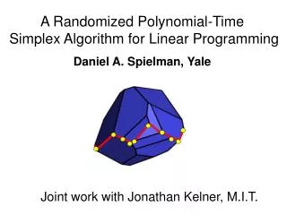
A Randomized Polynomial-Time Simplex Algorithm for Linear Programming. CS3150 Course Presentation. Linear Programming. Example: ・Find the maximum value of p = 3x - 2y + 4z ・subject to ・4x + 3y - z >= 3 ・x + 2y + z<=4 ・ x >= 0, y >= 0, z >= 0. Linear Programming.

E N D
A Randomized Polynomial-Time Simplex Algorithm for Linear Programming CS3150 Course Presentation
Linear Programming • Example: ・Find the maximum value of p = 3x - 2y + 4z ・subject to ・4x + 3y - z >= 3 ・x + 2y + z<=4 ・ x >= 0, y >= 0, z >= 0
Linear Programming • Objective Function max zT x • Constraints s.t. A x £ y
Simplex Method - Intuition • Objective: • Min C = 3x + 4y • Constraints: • ・3x - 4y <= 12, • ・x + 2y >= 4 • ・x >= 1, y >= 0.
Simplex Method - Intuition max zT x s.t. A x £ y • Worst-Case: exponential • Average-Case: polynomial • Widely used in practice
Shadow vertex pivot rule start z objective
Problem max zT x s.t. A x £ y The perturbed problem is no longer the original problem we want to solve! Solution Reduce the original problem to another problem, where the perturb won’t affect solution. Is this set of constraints bounded? A’w<=1 Some issues
Intuition of the Algorithm • Since the right hand side won’t affect solution, we want to carefully choose it so that the Shadow-Vertex Simplex will run poly-time with high probability.
Intuition of the Proof • P is the polytope of A’w<=1 • Case 1: • The polytope P is in k-near-isotropic position
Intuition of the Proof • Case 1: • The polytope is in k-near-isotropic position • Case 2: • The polytope is not in k-near-isotropic position
K-near-isotropic Case • Upper bound of total shadow length (Shadow Size). • Lower bound expected length of each edge. • Number of edges of the shadow is poly in size w.h.p.
Randomization • Each of vector is a independently exponentially distributed random variable with expectation • Project onto a random plane
None-K-near-isotropic Case • By Running the shadow vertex for a limited amount of time we can either: • Find the optimal • Or find a way to eliminate bad events w.h.p.
K-near-isotropic Case • Upper bound of the total shadow length. • Lower bound the expected length of each edge. • Number of edges of the shadow is poly in size w.h.p.
Upper Bound of Shadow Size • A’w<=1 • A’w<=1+r
Shadow Size in Case 1 • The expected shadow size is at most:
K-near-isotropic Case • Upper bound of the total shadow length. • Lower bound the expected length ofeach edge. • Number of edges of the shadow is poly in size w.h.p.
Expected Edge Length The Expected Edge Length is at least:
Case 1 Main Theorem • The expected number of edges is at most
None-K-Isotropic Case • The expected shadow size inside any given ball is small
None-K-near-Isotropic Case • Upper bound of the total shadow length within the given ball. • Lower bound the expected length of each edge within the given ball. • Number of edges of the shadow is poly in size w.h.p.
Outline of the Algorithm • Run Shadow Vertex Simplex on the Randomized Input • If Find Optimal then halt • Else transform the coordinates and run shadow vertex simplex on the transformed inputs • Algorithm will halt in poly-time w.h.p.
Summery and Intuitions • Deterministic algorithms run exponential time on some “bad” inputs • By introducing some randomness into the algorithm fixed the problem. • The Randomized algorithm run poly time on all inputs with high probability. • Start with something strict, which is easy to prove the poly-bound, eliminate the bad events in poly-time.