Download
1 / 17
170 likes | 183 Views
Oscillation Sensitivity. Jonathan Link Columbia University Braidwood Collaboration Meeting August 11, 2004. Study Parameters and Assumptions. Near detector located 200 meters from reactors on the surface. Far detectors at 1500 meters. Detector diameter is 6.5 meters

E N D
Oscillation Sensitivity Jonathan Link Columbia University Braidwood Collaboration Meeting August 11, 2004
Study Parameters and Assumptions • Near detector located 200 meters from reactors on the surface. • Far detectors at 1500 meters. • Detector diameter is 6.5 meters • 70 cm non-scintillating buffer (20 cm pmts & 50 cm to next layer) • 30 cm scintillating buffer • Detectors with & without scintillating buffer are considered
Detector Options Scintillating Buffer No Scintillating Buffer ~60 tons ~40 tons 30 cm 70 cm 6.5 meters No allowance is made for improved efficiency or increased target (from spill in effects) of the scintillating buffer design.
Study Parameters and Assumptions • Near detector located 200 meters from reactors on the surface. • Far detectors at 1500 meters. • Detector diameter is 6.5 meters • 70 cm non-scintillating buffer (20 cm pmts & 50 cm to next layer) • 30 cm scintillating buffer • Detectors with & without scintillating buffer are considered • Detector depth at 300 mwe or 450 mwe.
Background vs. Depth Non-spallation Backgrounds: At 300 mwe I took the Chooz Background rate of 0.2 /ton/day and assumed an improvement of a factor of 5 from having a flat overburden and improvements to the veto. At 450 mwe I assumed the a factor of two lower rate than 300 mwe (this is conservative).
Energy Dependence of the Background KamLAND Singles Distribution Fast Neutron Simulation Effective e+ energy from cosmic spallation neutron thermalization. For this study I used an exponential (e-E) plus flat background distribution. The fitter is free to vary the concentrations, but the input is 40% exp and 60% flat. A 50% normalization error is assumed. The shape fitter knows the exact form of the background contributions (Very Optimistic Assumption)
Correlated Decay Spallation Isotopes Correlated final state: β+n+2α Correlated final state: β+7Li Used Birks constant of 0.015 cm/MeV from Borexino (PLB 525, 29) for alphas and neutron thermalization (recoil protons)
Correlated Decay Spallation Isotopes (Cont.) • These are isotope production numbers. The correlated decay fraction is ½ or less. • I also assume: • 90% 9Li, 10% 8He • 20% normalization error on 9Li • 100% normalization error on 8He
Study Parameters and Assumptions • Near detector located 200 meters from reactors on the surface. • Far detectors at 1500 meters. • Detector diameter is 6.5 meters • 70 cm non-scintillating buffer (20 cm pmts & 50 cm to next layer) • 30 cm scintillating buffer • Detectors with & without scintillating buffer are considered • Detector depth at 300 mwe or 450 mwe. • Used either 1 near detector and 2 far or 2 near detectors and 4 far. • Assumed movable detectors.
Movable Detector Assumptions • I used 5% near running time for the calibration. • Therefore the relative error is given by • For 60 tons I get • σε = 0.34% from ~171,000 calibration events • And for 40 tons • σε = 0.42% from ~113,000 calibration events
Study Parameters and Assumptions • Near detector located 200 meters from reactors on the surface. • Far detectors at 1500 meters. • Detector diameter is 6.5 meters • 70 cm non-scintillating buffer (20 cm pmts & 50 cm to next layer) • 30 cm scintillating buffer • Detectors with & without scintillating buffer are considered • Detector depth at 300 mwe or 450 mwe. • Used either 1 near detector and 2 far or 2 near detectors and 4 far. • Assumed movable detectors. • Compared Counting only, Shape only and Counting+Shape Analyses.
First Observations Counting+Shape is the superior analysis, and Counting alone is better that Shape alone at these exposures. Shape dominance begins sometime between 3500 and 5000 GW ton years.
First Observations Counting+Shape is the superior analysis, and Counting alone is better that Shape alone at these exposures. Shape dominance begins sometime between 3500 and 5000 GW ton years. The transition point depends on the level systematic error. When backgrounds are increased we see that the big advantage in Shape+Counting over Counting alone comes from fitting the backgrounds.
Baseline Study The last baseline study that I did ignored the effects of backgrounds. The conclusion was that 1500 meters was not a bad place to be, but the counting experiment might do better if it was a little further back. For this study I looked only at the extrema of the exposure (1700 GW ton years and 5200 GW ton years) Background to signal increases by 50% from 1500 to 1800 m.
Baseline Study (Continued) Only for the smallest Δm2 is there any benefit to a longer baseline.
Conclusions and Future Work • I am now more strongly convinced that the optimal baseline is 1500 meters or less. • I need to extend the sensitivity study to less that 1500 meters. • The Counting sensitivity is very sensitive the level of background relative to signal. • This may also be true for the Shape analysis. • I need to include uncertainties in the background shape. • More far detector mass is better.