Download
1 / 44
460 likes | 649 Views
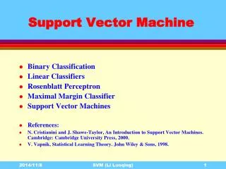
Lecture 10: Support Vector Machines. Machine Learning Queens College. Today. Support Vector Machines Note : we ’ ll rely on some math from Optimality Theory that we won ’ t derive. Maximum Margin. Are these really “ equally valid ” ?.

E N D
Lecture 10: Support Vector Machines Machine Learning Queens College
Today Support Vector Machines Note: we’ll rely on some math from Optimality Theory that we won’t derive.
Maximum Margin Are these really “equally valid”? • Linear Classifiers can lead to many equally valid choices for the decision boundary
Max Margin Small Margin Large Margin Are these really “equally valid”? • How can we pick which is best? • Maximize the size of the margin.
Support Vectors Support Vectors are those input points (vectors) closest to the decision boundary 1. They are vectors 2. They “support” the decision hyperplane
Support Vectors Define this as a decision problem The decision hyperplane: No fancy math, just the equation of a hyperplane.
Support Vectors • Aside: Why do some cassifiers use or • Simplicity of the math and interpretation. • For probability density function estimation 0,1 has a clear correlate. • For classification, a decision boundary of 0 is more easily interpretable than .5.
Support Vectors Define this as a decision problem The decision hyperplane: Decision Function:
Support Vectors Define this as a decision problem The decision hyperplane: Margin hyperplanes:
Support Vectors The decision hyperplane: Scale invariance
Support Vectors The decision hyperplane: Scale invariance
Support Vectors This scaling does not change the decision hyperplane, or the support vector hyperplanes. But we will eliminate a variable from the optimization The decision hyperplane: Scale invariance
What are we optimizing? • We will represent the size of the margin in terms of w. • This will allow us to simultaneously • Identify a decision boundary • Maximize the margin
How do we represent the size of the margin in terms of w? Proof outline: If not, we could define a larger margin support hyperplane that does touch the nearest point(s). There must at least one point that lies on each support hyperplanes
How do we represent the size of the margin in terms of w? Proof outline: If not, we could define a larger margin support hyperplane that does touch the nearest point(s). There must at least one point that lies on each support hyperplanes
How do we represent the size of the margin in terms of w? And: There must at least one point that lies on each support hyperplanes Thus:
How do we represent the size of the margin in terms of w? And: There must at least one point that lies on each support hyperplanes Thus:
How do we represent the size of the margin in terms of w? • The vector w is perpendicular to the decision hyperplane • If the dot product of two vectors equals zero, the two vectors are perpendicular.
How do we represent the size of the margin in terms of w? The margin is the projection of x1 – x2 onto w, the normal of the hyperplane.
How do we represent the size of the margin in terms of w? Projection: Size of the Margin: The margin is the projection of x1 – x2 onto w, the normal of the hyperplane.
Maximizing the margin Linear Separability of the data by the decision boundary Goal: maximize the margin
Max Margin Loss Function If constraint optimization then Lagrange Multipliers Optimize the “Primal”
Max Margin Loss Function Partial wrt b Optimize the “Primal”
Max Margin Loss Function Partial wrt w Optimize the “Primal”
Max Margin Loss Function Partial wrt w Now have to find αi. Substitute back to the Loss function Optimize the “Primal”
Max Margin Loss Function Construct the “dual”
Dual formulation of the error There exist (rather) fast approaches to quadratic program solving in both C, C++, Python, Java and R Solve this quadratic program to identify the lagrange multipliers and thus the weights
Quadratic Programming • If Q is positive semi definite, then f(x) is convex. • If f(x) is convex, then there is a single maximum.
Support Vector Expansion New decision Function Independent of the Dimension of x! When αi is non-zero then xi is a support vector When αi is zero xi is not a support vector
Karush-Kuhn-Tucker Conditions Only points on the decision boundary contribute to the solution! • In constraint optimization: At the optimal solution • Constraint * Lagrange Multiplier = 0
Interpretability of SVM parameters • What else can we tell from alphas? • If alpha is large, then the associated data point is quite important. • It’s either an outlier, or incredibly important. • But this only gives us the best solution for linearly separable data sets…
Basis of Kernel Methods The decision process doesn’t depend on the dimensionality of the data. We can map to a higher dimensionality of the data space. Note: data points only appear within a dot product. The error is based on the dot product of data points – not the data points themselves.
Basis of Kernel Methods • Since data points only appear within a dot product. • Thus we can map to another space through a replacement • The error is based on the dot product of data points – not the data points themselves.
Learning Theory bases of SVMs • Theoretical bounds on testing error. • The upper bound doesn’t depend on the dimensionality of the space • The lower bound is maximized by maximizing the margin, γ, associated with the decision boundary.
Why we like SVMs • They work • Good generalization • Easily interpreted. • Decision boundary is based on the data in the form of the support vectors. • Not so in multilayer perceptron networks • Principled bounds on testing error from Learning Theory (VC dimension)
SVM vs. MLP • SVMs have many fewer parameters • SVM: Maybe just a kernel parameter • MLP: Number and arrangement of nodes and eta learning rate • SVM: Convex optimization task • MLP: likelihood is non-convex -- local minima
Soft margin classification • There can be outliers on the other side of the decision boundary, or leading to a small margin. • Solution: Introduce a penalty term to the constraint function
Soft Max Dual Still Quadratic Programming!
Soft margin example Hinge Loss Points are allowed within the margin, but cost is introduced.
Probabilities from SVMs • Support Vector Machines are discriminant functions • Discriminant functions: f(x)=c • Discriminative models: f(x) = argmaxcp(c|x) • Generative Models: f(x) = argmaxcp(x|c)p(c)/p(x) • No (principled) probabilities from SVMs • SVMs are not based on probability distribution functions of class instances.
Efficiency of SVMs • Not especially fast. • Training – n^3 • Quadratic Programming efficiency • Evaluation – n • Need to evaluate against each support vector (potentially n)
Next Time Perceptrons