Download

1 / 22
220 likes | 364 Views
The Market. Supply & Demand & all that. The Big Picture. P. P. Q. Q. Demand. Supply. P. Equilibrium Price & Quantity. Q. The Market. Demand. Analysis based on individuals' behavior, then summing of individuals into aggregate demand at various prices Explanations

E N D
The Market Supply & Demand & all that
The Big Picture P P Q Q Demand Supply P Equilibrium Price & Quantity Q The Market
Demand • Analysis based on individuals' behavior, then summing of individuals into aggregate demand at various prices • Explanations • Verbal: quantity demanded changes inversely w/price • Simple graph: downward sloping curve of P vs Q • Graphic derivation: from preferences • Mathematical specification: D = f(P) • Axiomatic derivation
Indifference Curves - I Two space defines various combinations of Q1 & Q2 that you might choose. Some (Q1, Q1) you prefer to others, some you prefer less, some alternatives leave you indifferent. An “indifference curve” is defined by set of combinations among which you are indifferent. I1 < I2 < I3 Quant. of Good 2 Dem. (Q2) higher levels of preference higher levels of utility q" q' q P1 O Quantity of Good 1 Demanded (Q1) NB: under usual assumptions: 1. Q1 and Q2 are infinitely divisible, so: infinite # of smooth curves 2. curves are open, I.e., you always prefer MORE of everything
Indifference Curves - II I1 < I2 < I3 Quant. of Good 2 Dem. (Q2) q" q' q P1 O Quantity of Good 1 Demanded (Q1) NB: if you drop the assumption that you always prefer MORE of everything, then at some point curves close, and MORE would mean a lower level of utility
Budget Line - I Available budget (money) = M with prices of Q1 = P1, Q2 = P2 so, total expenditure = M = P1Q1+P2Q2 which defines the “budget line.” Q2 q2 If all M spent on Q2 then you would be at q2. If all M spent on Q1 then you would be at q1. NB: if you spend less than M, you will be at some point under the budget line in the space defined by 0,q1,q2. q1 Q1 O If you rewrite M = P1Q1+P2Q2 as Q2 = (1/P2)M - (P1 / P2) Q1 you can see that the slope of the line = P1/ P2 (and is negative)
Budget Lines - IIIf income (M) increases, budget line shifts right Q2 M' =P1Q1+P2Q2 M=P1Q1+P2Q2 P1 Q1 O If M' > M, then line shifts right.
Budget Lines - IIIIf P1 increases, budget line intercept shifts left Q2 If P1 increases, max Q1 falls (Change in P1 would have no effect on vertical intercept if all M spent on Q2) Q1 O If P1<P1’, then intercept shifts left. If P2/P1 changes, slope changes
Utility Maximization I3 Q2 M=P1Q1+P2Q2 Q1 q O To Maximize utility you will want to be on highest possible I. Highest possible I will be that which is tangent to budget line.
Graphic Derivation of Demand CurveDemand Curve shows what happens to quantity demanded as price changes. So we raise P1 and see what happens to Q1 I1 < I2 < I3 P1" P1' P1' P1 P1 P1" q" q' q q" q' q O Quantity of Good 1 Demanded (Q1) As price rises, P1< P1'< P1”, quantity demanded falls, q to q’ to q” and the combinations of P1 and q define a demand curve for Q1.
Mathematical Specificationof Demand Curves D = f(P) dD/dP < 0 D/P < 0 Linear Demand Functions D = a - bP D = 300 - 20P
Axiomatic Derivation • Subset of Assumptions • A > B, A < B, A = B • axiom of transitivity • axiom of asymmetry • comparability • egotism, no one else's consumption matters to you • continuity (continuous curves, eg., indifference curves • insatiability (no maximium, always want more)
Utility • Indifference Curves defined by: • preference - further from origin prefered • utility - further from origin, higher utility • Utility = satisfaction derived from consumption • Utility derived from "utilitarians" - Eng. Philos. • all action taken with view to utility to be derived • measured by "utils"cardinality • law of diminishing marginal utility (maybe!) • Utility functions: U = f(x1, x2, .... xn)
Problem w/utility • Cardinality • you can compare utility for different people • interpersonal comparisons • Law of Diminishing Mar. Utility • how much utility depended upon how much you have • Cardinality + Law of Diminishing Utility • total social utility would increase through redistribution of money from rich to poor • a political problem! Solution: shift to ordinality( ±) • utility theory replaced by preference theory
Supply • Analysis based on each firm's behavior, then summing of firms into aggregate supply at various prices • Explanations • Verbal: quantity supplied changes directly w/price • Simple graph: upward sloping curve of P vs Q • Graphic derivation: from costs + profit maximization • Mathematical specification: S = f(P) • Axiomatic derivation
Costs Price, costs Marginal cost (MC) average cost price given = marginal revenue (MR) quantity produced Profit Maximization occurs where MC = MR
Derivation of Supply Curve Price, costs Marginal cost (MC) = S P3 P2 P1 q1 q2 q3 quantity produced Profit Maximization occurs where MC = MR
Mathematical Specification S = f(P) dS/dP > 0 S/P > 0 Linear Supply Functions S = a + bP S = 300 + 20P
Axiomatic Derivation • Subset of axioms • Existence of Production • There exists some attainable element x that can be transformed into y • Neutrality of Transformations • any two transformations T are indifferenttheir inputs are indifferent and their outputs are indifferent • Convexity • Production set Yj is convex
Change in Technology • Improvements in Technology that lower costs of production, shift MC curve down, and Supply curve to Right MC/S MC'/S' Supply shifts to the right marginal cost shifts down
Equilibrium • Shapes of S & D guarantee "equilibrium", i.e., tendency to return to price that equalizes them Supply P excess supply equilibrium price Demand Q equilibrium quantity