Download
1 / 20
200 likes | 340 Views
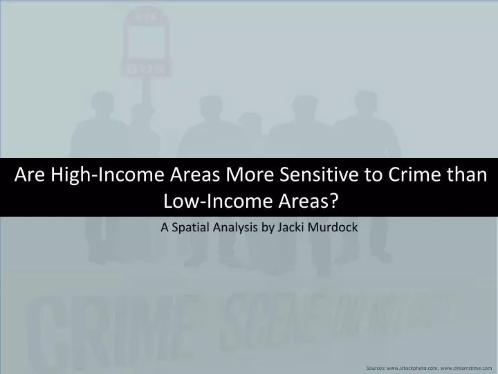
Are High-Income Areas More Sensitive to Crime than Low-Income Areas?. A Spatial Analysis by Jacki Murdock. Sources: www.istockphoto.com; www.dreamstime.com. In the midterm we discovered that transit use in low income areas is not significantly impacted by crime .

E N D
Are High-Income Areas More Sensitive to Crime than Low-Income Areas? A Spatial Analysis by Jacki Murdock Sources: www.istockphoto.com; www.dreamstime.com
In the midterm we discovered that transit use in low income areas is not significantly impacted by crime. • However, this may be because the site selected was transit dependent, and therefore was not as sensitive to crime because they do not have access to another mode of travel. • So, is transit use more affected by crime (i.e. more sensitive to crime) in higher income areas compared with lower income areas? • I chose two sites based on the Los Angeles Times “mapping LA” site’s median income data: Hancock Park and Watts. • Data: METRO bus ridership data for every month (September 2011-January 2012) LAPD crime data for those months LA Times Mapping LA, ESRI, 2010 TIGER, MIT GIS Services The Question
Hancock Park Watts • 6,459 people per square mile • 71% White • 13% Asian • $85,277 Median Income • 56.2% have a four year degree • 25 Crimes in October, 2011 • 55 Bus Stops • 17,346 people per square mile • 62% Latino • 37% Black • $25,161 Median Income • 2.9% have a four year degree • 48 Crimes in October, 2011 • 76 Bus Stops
Process of Site Selection In order to determine if higher income, less transit dependent communities were more sensitive to crime than lower income, transit dependent communities, I chose a higher and lower income area based on the LATimes Crime Mapping rankings of neighborhoods. Hancock Park Watts
Total Ridership and Crime: Watts Total Ridership and Crime: Hancock Park 105 Freeway Wilshire Boulevard
The Mean Center represents the shortest average distance from crime or ridership. In Watts, the average distance between crime and average distance between bus riders is shorter than in Hancock Park . Mean Center: Watts Mean Center: Hancock 105 Freeway Wilshire Boulevard
This circle represents one standard deviation from the mean. 66% of crime and ridership happen within these circles. So, the smaller the circle, the more clustered the crime/ridership. Much of the ridership in Watts overlaps with most of the crime incidents, whereas most of the crime/ridership does not intersect in Hancock Park Standard Distance: Watts Standard Distance: Hancock 105 Freeway Wilshire Boulevard
The standard distance assumes a normal distribution of features within the circle. However, this is very rarely the case. This measure shows the direction and the distribution of crime and ridership. In Hancock park, riders are much less distributed than in Watts. Yet Crime seems to be similarly distributed. Standard Deviation Ellipse: Watts Standard Deviation Ellipse: Hancock 105 Freeway Wilshire Boulevard
Next, I ran a spatial autocorrelation test to see if the general pattern of features is clustered or dispersed. In the Moran’s Index, the higher the value, the more clustered. Crime and Ridership are clustered in both Watts and Hancock Park *All of the variables had statistically significant results at P-values below 0.05.
To know more about why crime and ridership are clustered, I performed a Hot Spot Analysis Crime Incidents Hot Spot: Hancock Park Transit Ridership Hot Spot: Hancock Park Wilshire Boulevard Wilshire Boulevard Wilshire Boulevard
The Hot Spots, in red, are surrounded around high levels of ridership/crime. In addition, they are surrounded around more ridership/crime than its neighbors. This may be way Watts has no significant hot spots, because high crime levels occur more dispersedly. Crime Incidents Hot Spot: Watts Transit Ridership Hot Spot: Watts 105 Freeway 105 Freeway
Next, I used Network Analyst to find the average distance to crime for each transit stop. Then, I ran an OLS Regression to find out where stops proximity to crime was effecting ridership. Average Distance to Crime and Ridership: Watts Average Distance to Crime and Ridership: Hancock Park Wilshire Boulevard 105 Freeway
Next, I used Network Analyst to find the average distance to crime for each transit stop. Then, I ran an OLS Regression to find out where stops proximity to crime was effecting ridership. Average Distance to Crime and Ridership: Watts Average Distance to Crime and Ridership: Hancock Park Wilshire Boulevard 105 Freeway
R-Squared tells us how well the regression was able to predict crimes’ effect on transit use. In our case, the R-squared is extremely low in both cases, but is slightly higher in Watts, possibly due to its higher incidents of crime. *All of the variables had statistically significant results at P-values below 0.05.
Implications • We have seen that there are significant differences in sensitivity to crime between a high-income and low-income area. • Watts is not as sensitive to crime as is Hancock Park • Presumably, this is because those transit stops where most crime occurs in Hancock Park are not used as often because their residents have access to vehicles, while many Watts’ residents do not.
Inset Map • Graduated Symbols • Aggregating Attribute Fields • Attribute sub-set selections • Geographic sub-set selections • Geoprocessing • Geocoding • Charts • Network Analyst (to find average distance to crime for each transit stop) • 5 Models • Spatial Statistics (Mean Center, Standard Distance, Standard Deviation Ellipse, Getis-Ord General Gi, Spatial Autocorrelation, OLS Regression) Skills Used