Download
1 / 35
360 likes | 433 Views
Sampling Distributions. Chapter 9. Introduction . In this chapter we study some relationships between population and sample characteristics. Generally, we are interested in population parameters such as Mean return Variability of demand Proportion of defectives in a production line.

E N D
Sampling Distributions Chapter 9
Introduction • In this chapter we study some relationships between population and sample characteristics. • Generally, we are interested in population parameters such as • Mean return • Variability of demand • Proportion of defectives in a production line
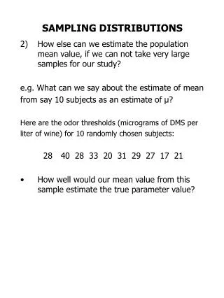
Introduction • Such parameters are usually unknown • Therefore, we draw a samples from the population, and use them to make inference about the parameters. • This is done by constructing sample statistics, that have close relationship to the population parameters.
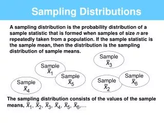
Introduction • Samples are random, so the sample statistic is a random variable. • As such it has a sample distribution. • Sample distributions for various statistics are studied in this chapter
x 1 2 3 4 5 6 p(x) 1/6 1/6 1/6 1/6 1/6 1/6 9.1 Sampling Distribution of the Mean • Example 1 • A die is thrown infinitely many times. Let X represent the number of spots showing on any throw. • The probability distribution of X is E(X) = 1(1/6) + 2(1/6) + 3(1/6)+ ………………….= 3.5 V(X) = (1-3.5)2(1/6) + (2-3.5)2(1/6) + …………. …= 2.92
Throwing a die twice – sample mean • Suppose we want to estimate m from the mean of a sample of size n = 2. • What is the distribution of ?
Throwing a die twice – sample mean And these are the means of each pair These are all the possible pairs of values for the 2 throws
(1+3)/2 = 2 (2+2)/2 = 2 (3+1)/2 = 2 (1+1)/2 = 1 (1+2)/2 = 1.5 (2+1)/2 = 1.5 Notice there are 36 possible pairs of values: 1,1 1,2 ….. 1,6 2,1 2,2 ….. 2,6 ……………….. 6,1 6,2 ….. 6,6 The distribution of when n = 2 Calculating the relative frequency of each value of we have the following results • 1.5 2.0 2.5 3.0 3.5 4.0 4.5 5.0 5.5 6.0 • 1 2 3 4 5 6 5 4 3 2 1 • 1/36 2/36 3/36 4/36 5/36 6/36 5/36 4/36 3/36 2/36 1/36 Frequency Relative freq
The Relationship between the sample size and the sampling distribution of the sample mean As the sample size changes, the mean of the sample mean does not change!
The Relationship between the sample size and the sampling distribution of the sample mean As the sample size increases, the variance of the sample mean decreases!
The Relationship between the sample size and the sampling distribution of the sample mean Also, note the interesting relationship between the sample size and the variance of the sample mean. We’ll formalize this relationship soon.
The Sample Variance Demonstration: Why is the variance of the sample mean is smaller than the population variance. Mean = 1.5 Mean = 2. Mean = 2.5 1.5 2.5 Population 2 1 2 3 Compare the range of the population to the range of the sample mean. Let us take samples of two observations. Click
The Central Limit Theorem • If a random sample is drawn from any population, the sampling distribution of the sample mean is: • Normal if the parent population is normal, • Approximately normal if the parent population is not normal, provided the sample size is sufficiently large. • The larger the sample size, the more closely the sampling distribution of will resemble a normal distribution.
The mean of X is equal to the mean of the parent population The variance of X is equal to the parent population variance divided by ‘n’. The Parameters of theSampling Distribution of X
The Sampling Distribution of X - Example • Example 2 • The amount of soda pop in each bottle is normally distributed with a mean of 32.2 ounces and a standard deviation of .3 ounces. • Find the probability that a bottle bought by a customer will contain more than 32 ounces.
m = 32.2 x = 32 The Sampling Distribution of X - Example • Example 2 SolutionThe random variable X is the amount of soda in a bottle. 0.7486
The Sampling Distribution of X • Find the probability that a carton of four bottles will have a mean of more than 32 ounces of soda per bottle. • Solution • Define the random variable as the mean amount of soda per bottle. 0.9082
The Sampling Distribution of X • Example 3 • The average weekly income of B.B.A graduates one year after graduation is $600. • Suppose the distribution of weekly income has a standard deviation of $100. What is the probability that 35 randomly selected graduates have an average weekly income of less than $550? • Solution
The Sampling Distribution of X • Example 3 – continued • If a random sample of 35 graduates actually had an average weekly income of $550, what would you conclude about the validity of the claim that the average weekly income is 600? • Solution • With m = 600 the probability to have a sample mean as low as 550 is very small (0.0015). The claim that the mean weekly income is $600 is probably unjustified. • It will be more reasonable to assume that m is smaller than $600, because then a sample mean of $550 becomes more probable.
9.2 Sampling Distribution of a Sample Proportion (p) < • The parameter of interest for qualitative (nominal) data is the proportion of times a particular outcome (success) occurs for a given population. • This is the motivation for studying the distribution of the sample proportion
p The number of successes X n = < 9.2 Sampling Distribution of a Sample Proportion (p) • Let X be the number of times an event of interest takes place (we can call such an event a success just like the definition we used for the binomial experiment) The sample proportion = <
p 9.2 Sampling Distribution of a Sample Proportion (p) < • Since X is binomial, probabilities for can be calculated from the binomial distribution. • Yet, for inference about we prefer to use normal approximation to the binomial. < < p
Approximate Sampling Distribution of a Sample Proportion • From the laws of expected value and variance, it can be shown that m = p and s2 = p(1-p)/n • Z is calculated by: • If both np > 5 and n(1-p) > 5, then Z is approximately standard normal.
Approximate Sampling Distribution of a Sample Proportion • Example 5 • A state representative received 52% of the votes in the last election. • One year later the representative wanted to study his popularity. • If his popularity has not changed, what is the probability that more than half of a sample of 300 voters would vote for him?
Approximate Sampling Distribution of a Sample Proportion • Example 5 • Solution • The number of respondents who prefer the representative is binomial with n = 300 and p = .52. Thus, np = 300(.52) = 156 > 5n(1-p) = 300(1-.52) = 144 > 5. The normal approximation can be applied here:
Using Sampling Distributions for Inference • Sampling distributions can be used to make an inference about population parameters • For example let us look at an inference about the population mean • Generally we’ll compare the actual sample mean with a hypothesized value of the unknown population mean, and make an informed decision about the likelihood of this hypothesis
Large probability that falls inside [m-D, m+D] m - Dm + D Using Sampling Distributions for Inference • Let us guess what the value of m is, and build a symmetrical interval around m large enough to make it very likely that the sample mean falls inside it. • If the sample mean falls outside the interval (although this is very unlikely), we tend to believe that m is different than the value of m we guessed. • The sampling distribution of the sample mean helps in performing the calculations. m
Using Sampling Distributions for Inference Suppose .95 is considered sufficiently large probability the sample mean falls inside the interval. Let us build a symmetrical interval around m. Using the notation m - D and m + D we have: P(m - D £ £ m + D) = .95.
Using Sampling Distributions for Inference Performing the usual standardization we find that the interval covering 95% of the distribution of the sample mean is: 0.95
Using Sampling Distributions for Inference • Conclusion • There is 95% chance that the sample mean falls within the interval [560.8, 639.2] if the population mean is 600. • Since the sample mean was 550, the population mean is probably not 600. Now let us apply this interval to example 3.
Optional: Sampling Distribution of the Difference Between Two Means • The difference between two means can become a parameter of interest when the comparison between two populations is studied. • To make an inference about m1 - m2 we observe the distribution of .
If the two populations are not both normally distributed, but the sample sizes are 30 or more, the distribution of is approximately normal. 9.3 Normal Distribution of the Difference Between two Sample Means • The distribution of is normal if • The two samples are independent, and • The parent populations are normally distributed.
We can define: 9.3 Normal Distribution of the Difference Between two Sample Means • Applying the laws of expected value and variance we have:
9.3 Normal Distribution of the Difference Between two Sample Means Example 6 The starting salaries of MBA students from two universities (WLU and UWO) are $62,000 (stand.dev. = $14,500), and $60,000 (stand. dev. = $18,300). • What is the probability that a sample mean of WLU students will exceed the sample mean of UWO students? (nWLU = 50; nUWO = 60)
9.3 Normal Distribution of the Difference Between two Sample Means • Example 6 – Solution We need to determine m1 - m2 = 62,000 - 60,000 = $2,000